因子分析

因子分析（factor analysis）はデータの分散を分解することによって何らかの共通性を抽出する手法である。

心理学などの分野において、「リーダシップ」や「社交性」のような直接観測することができない構成概念（construct）を抽出するために用いられる。

ビジネスにおいてはどういったところで応用されるのか？¶

心理学以外の利用例

因子分析モデル¶

1因子モデル¶

$p$ 次元の観測値が $n$ 個得られているとし、 $i$ 番目の $j$ 次元のデータを $x_{ij}$ と表すことにする。 $x_{ij}$ を標準化して平均0、分散1にしたデータを $z_{ij}$ と表すことにする。

1因子モデルは標準化データを次のように分解するモデルである。

独自因子・独自係数は誤差項 $e$ としてまとめる表記

z_{ij} = a_j f_i + e_{ij}

(2)

も存在する。独自因子と独自係数はどちらも自由に推定しようとすると解が定まらない（ $d_j$ を2倍にして $u_{ij}$ を半分にしてもいい）ので、推定の際は通常は $d_j=1$ に固定する。

1因子モデルをベクトルで表すと次のようになる

因子スコア $f_{i}$ が観測対象（アンケート回答者など）ごとに算出されるため、個々の観測対象のスコアリングができる。

$m$ 因子モデル¶

$m$ 個の因子を扱うように拡張した場合は次のように表される。

ベクトルの場合は

\begin{aligned} \mathbf{z}_j &= a_{j1} \mathbf{f}_1 + a_{j2} \mathbf{f}_2 + \cdots + a_{jm} \mathbf{f}_m + \mathbf{e}_j \\ &= \begin{pmatrix} \mathbf{f}_1 & \mathbf{f}_2 & \cdots & \mathbf{f}_m \end{pmatrix} \begin{pmatrix} a_{j1} \\ a_{j2} \\ \vdots \\ a_{jm} \end{pmatrix} + \mathbf{e}_j \\ &= \mathbf{F} \mathbf{a}_j + \mathbf{e}_j \end{aligned}

(5)

と表すことができる。

因子分析モデル（行列表現）¶

観測値ごとの添字をつけると $i \times j \times l$ で3方向の次元（テンソル）になってしまうので簡略化のため観測値ではなく確率変数として扱うと、よりシンプルなモデルになる。

設問項目（item）が $I$ 個あり、 $I$ 個の確率変数 $x_1,\dots,x_I$ が得られたとする。それを平均0分散1へと標準化したものを $z_1,\dots,z_I$ とする。これらが $T$ 個の因子（trait）から影響を受けていると仮定し、 $T$ 個の共通因子 $f_1,\dots,f_T$ と因子負荷量 $\lambda_{11},\lambda_{12},\dots,\lambda_{IT}$ で

z_i = \lambda_{i1} f_1 + \cdots + \lambda_{iT} f_T + \varepsilon_i \quad (i = 1,\dots, I)

(6)

と説明する線形モデルが因子分析モデルとなる。行列とベクトルで表すと次のようになる

また、共通因子 $\mathbf{f}$ と独自因子 $\mathbf{\varepsilon}$ には次の仮定がおかれる：

$\mathbf{f}$ と $\mathbf{\varepsilon}$ は統計的に独立
$\operatorname{E}[\mathbf{f}] = 0, \quad \operatorname{Var}[\mathbf{f}] = \mathbf{\Phi}$
$\operatorname{E}[\boldsymbol{\varepsilon}] = 0, \quad \operatorname{Var}[\boldsymbol{\varepsilon}] = \mathbf{\Psi}$
- （ $\mathbf{\Psi}$ は対角行列、つまり異なる変数に対する独自因子は無相関とする）

この仮定により、観測変数の分散共分散行列を考えると

\operatorname{Var}[\mathbf{z}] =\mathbf{\Sigma} =\mathbf{\Lambda \Phi \Lambda^\top} + \mathbf{\Psi}

(8)

となる。つまり、 観測された変数の分散共分散行列をモデルのパラメータで説明するモデル であることがわかる。

$\mathbf{z}$ を中心化ではなく標準化している場合、分散共分散行列ではなく相関係数行列に対して上記の構造化を考えることになる。

（参考：因子分析 - Wikipedia）

パラメータの推定¶

因子分析モデルのパラメータは観測変数の相関行列をもとにして最尤推定法などで推定される。

$\mathbf{\Lambda}, \mathbf{\Psi}$ の推定（最尤推定法による例）¶

標本共分散行列 $\mathbf{S}$ を使って、尤度関数は

\mathcal{L}(\mathbf{\Lambda}, \mathbf{\Psi})=-\frac{n}{2}(\log |\mathbf{\Sigma}|+\operatorname{tr}(\mathbf{S} \mathbf{\Sigma}^{-1}))

(9)

と表される。これをEMアルゴリズムなどで最大化して $\mathbf{\Lambda}, \mathbf{\Psi}$ の推定値を得る。

$\mathbf{f}$ の推定（バートレット法による例）¶

最小二乗法にちょっと似てる数式で、独自因子の分散の逆行列で重み付け（誤差が大きい場合はスコアへの寄与が小さくなる）を行いつつ推定する

\hat{\mathbf{f}}=\left(\boldsymbol{\Lambda}^{\top} \mathbf{\Psi}^{-1} \boldsymbol{\Lambda}\right)^{-1} \boldsymbol{\Lambda}^{\top} \mathbf{\Psi}^{-1} \mathbf{x}

(10)

実装例¶

import pandas as pd

# テストの点数データ
scores = pd.DataFrame([
    {"英語": 98, "国語": 95, "数学": 75},
    {"英語": 90, "国語": 75, "数学": 70},
    {"英語": 60, "国語": 57, "数学": 80},
    {"英語": 50, "国語": 70, "数学": 60},
    {"英語": 30, "国語": 50, "数学": 40},
])
Z = (scores - scores.mean()) / scores.std()

from statsmodels.multivariate.factor import Factor

fa = Factor(Z, n_factor=1, method="ml").fit()
fa.summary()

/usr/local/lib/python3.10/site-packages/statsmodels/multivariate/factor.py:417: UserWarning: Fitting did not converge
  warnings.warn("Fitting did not converge")

Loading...

fa.uniqueness

array([0.00228581, 0.22772564, 0.46534024])

# 共通因子スコア
fa.factor_scoring(Z)

array([[ 1.15171807],
       [ 0.85998399],
       [-0.19932969],
       [-0.54814633],
       [-1.26422604]])

主成分分析との違い¶

主成分分析も分散を分解して共通した成分を取り出す手法であり、因子分析と似ているが、誤差を分離するかどうかが異なる。

因子分析は観測変数を共通した部分と誤差とに分解した上で共通因子を抽出するのに対し、主成分分析は誤差の分離を行わずに共通した部分を取り出そうとする。

妥当性と信頼性¶

信頼性係数¶

真の得点の分散の、テスト得点の分散に対する比を、テスト得点 $y$ の 信頼性係数 (reliability coefficient) という。

\rho=\frac{\sigma_t^2}{\sigma_y^2} =\frac{\sigma_t^2}{\sigma_t^2+\sigma_e^2}=1-\frac{\sigma_e^2}{\sigma_y^2}

(11)

信頼性係数は測定の誤差分散が小さいほど1に近い値をとり、誤差分散が大きいとき0に近い値をとる。

クロンバックの $\alpha$ 係数¶

信頼性係数 $\rho$ は母集団レベルの話であり、標本の情報から推定するには別の値を使う。信頼性係数の推定方法はいくつかあるが、「項目を超えた一貫性」に関する検討を行うクロンバックのα係数が代表的。

「項目を超えた一貫性」とは「テストに含まれる項目群を、同様の別の項目群に置き換えても結果は安定しているか」という考え方で、そういう意味での信頼性を近似的に与える指標がクロンバックのα係数である。

クロンバックの

\alpha

\alpha=\frac{J}{J-1}\left(1-\frac{\sum_{j=1}^J s_j^2}{s_y^2}\right)

(12)

$J$ ：項目数
$s_y^2$ ：テスト得点の分散
$s_j^2$ ：項目 $j$ の分散

$\alpha$ 係数は

項目間の相関が高いとき
項目数が多いとき

に高い値をとる。項目が多いだけでも高くなってしまうので注意が必要で参考程度に用いられる。

測定の標準誤差（SEM）は信頼性係数の推定値 $\hat\rho$ を用いて推定される。

測定の標準誤差（SEM）の推定量

\operatorname{SEM} = s_y \sqrt{1-\hat{\rho}}

(13)

Messickの妥当性概念¶

Messickは妥当性検証のための側面を6つ挙げた。

側面（facet）	内容（簡潔な説明）
① 内容的妥当性（Content）	測定内容が理論的構成概念をどれだけ網羅しているか
② 構成概念妥当性（Substantive）	測定が理論に基づき、認知的に妥当か
③ 構造的妥当性（Structural）	得点構造が想定した構成概念と整合しているか（因子構造など）
④ 外的妥当性（External）	他の指標との関係が理論通りか（収束的・弁別的妥当性）
⑤ 結果的妥当性（Consequential）	測定の利用が社会的に望ましい結果をもたらすか（公正性・偏りなど）
⑥ 実証的妥当性（Generalizability）	測定結果が一般化可能か（状況・集団を超えて妥当か）

上記6つの側面にわたる証拠が備えられていることが望ましい。しかし妥当性検証とは尺度が利用されることで明らかになる証拠を積み重ねるプロセスであるため、最初から全部を備えることは不可能。

探索的因子分析¶

探索的因子分析（exploratory factor analysis: EFA）は、因子と観測変数の関係についての仮説や制約を置かずに、観測変数のみから相関係数を計算し、観測変数間に相関関係をもたらす因子を推定する方法。

たとえばモデルの因子の数は固有値から探索して決める。例えば「1より大きい固有値をもつ因子を採用する」とする（Guttman基準）

サンプルデータを生成して因子分析を実行してみる¶

import numpy as np
import pandas as pd

def generate_factor_analysis_data(n_samples=1000, n_variables=3, noise_std=0.1, random_state=42):
    """因子分析のサンプルデータを生成する"""
    np.random.seed(random_state)
    n_factors = 1 # 1因子モデル

    # 因子負荷量行列（loadings）: n_variables × n_factors
    # loadings = np.random.uniform(0.5, 0.9, size=(n_variables, n_factors))
    loadings = np.array([
        [0.9],
        [0.5],
        [0.1],
    ])

    # 潜在因子スコア（factors）: n_samples × n_factors
    factors = np.random.normal(size=(n_samples, n_factors))

    # ノイズ項（ユニーク性）： n_samples × n_variables
    noise = np.random.normal(scale=noise_std, size=(n_samples, n_variables))

    # 観測変数: n_samples × n_variables
    data = factors @ loadings.T + noise

    # データフレームに変換
    columns = [f"X{i+1}" for i in range(n_variables)]
    df = pd.DataFrame(data, columns=columns)
    return df, factors, loadings

# サンプルデータ生成
df, true_factors, true_loadings = generate_factor_analysis_data()

display(pd.DataFrame(true_factors).head().style.set_caption("真の因子スコアの最初の5行"))
display(pd.DataFrame(true_loadings).style.set_caption("因子負荷量"))
display(df.head().style.set_caption("サンプルデータの最初の5行"))

Loading...

statsmodelsパッケージでの推定¶

from statsmodels.multivariate.factor import Factor
fa = Factor(endog=df, n_factor=1, method="ml").fit()
fa.rotate("promax")
fa.summary()

/usr/local/lib/python3.10/site-packages/statsmodels/multivariate/factor_rotation/_gpa_rotation.py:101: RuntimeWarning: divide by zero encountered in log10
  table.append([i_try, f, np.log10(s), al])

Loading...

factors_ = fa.factor_scoring(df)
display(pd.DataFrame(factors_).head().style.set_caption("因子スコアの最初の5行"))

Loading...

factor-analyzerパッケージでの推定¶

from factor_analyzer import FactorAnalyzer
fa = FactorAnalyzer(n_factors=1, rotation='promax', method='ml', is_corr_matrix=False)
fa.fit(df)

# 因子負荷量（loadings）
loadings = pd.DataFrame(fa.loadings_, index=df.columns, columns=["第1因子"])
loadings.style.set_caption("因子負荷量")

/usr/local/lib/python3.10/site-packages/sklearn/utils/deprecation.py:151: FutureWarning: 'force_all_finite' was renamed to 'ensure_all_finite' in 1.6 and will be removed in 1.8.
  warnings.warn(
/usr/local/lib/python3.10/site-packages/factor_analyzer/factor_analyzer.py:663: UserWarning: No rotation will be performed when the number of factors equals 1.
  warnings.warn(

Loading...

# 相関行列を渡す場合
from factor_analyzer import FactorAnalyzer
fa = FactorAnalyzer(n_factors=1, rotation='promax', method='ml', is_corr_matrix=True)
fa.fit(df.corr())

# 因子負荷量（loadings）
loadings = pd.DataFrame(fa.loadings_, index=df.columns, columns=["第1因子"])
loadings.style.set_caption("因子負荷量")

/usr/local/lib/python3.10/site-packages/sklearn/utils/deprecation.py:151: FutureWarning: 'force_all_finite' was renamed to 'ensure_all_finite' in 1.6 and will be removed in 1.8.
  warnings.warn(
/usr/local/lib/python3.10/site-packages/factor_analyzer/factor_analyzer.py:663: UserWarning: No rotation will be performed when the number of factors equals 1.
  warnings.warn(

Loading...

固有値を高い順に並べる スクリープロット

# スクリープロットで因子数を探索
import matplotlib.pyplot as plt
import matplotlib_fontja

eigen = fa.get_eigenvalues()
left = list(range(1, len(eigen[0])+1))
fig, ax = plt.subplots()
ax.plot(left, eigen[0], marker="o")
ax.set(xlabel="因子数（固有値の数）", ylabel="固有値", title="スクリープロット")
ax.axhline(y=1, color="gray", linestyle="--", alpha=0.5)
fig.show()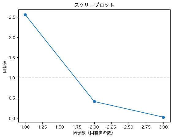

scikit-learnの因子分析¶

# 2因子モデルで因子分析を実行（scikit-learn）
from sklearn.preprocessing import StandardScaler
scaler = StandardScaler()
X_std = scaler.fit_transform(df)

from sklearn.decomposition import FactorAnalysis
fa = FactorAnalysis(n_components=1, random_state=0, rotation="varimax")
fa.fit(X_std)

# 因子スコア
factors_ = fa.transform(X_std)

# 因子負荷量（loadings）
loadings_ = pd.DataFrame(fa.components_.T, index=df.columns, columns=["第1因子"])  # shape: (n_variables, n_factors)
loadings_.style.set_caption("因子負荷量")

Loading...

plt.scatter(true_factors, factors_)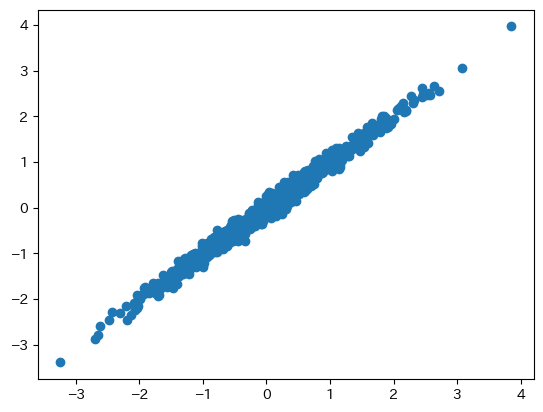

確認的因子分析¶

確認的因子分析（confirmatory factor analysis: CFA）は、因子の数や観測変数との関係性などについての仮説（モデル）をあらかじめ立てておき、その仮説の正しさを検証するためにモデルをデータにあてはめていく。

その妥当性はデータの分散をモデルがどれだけ説明できたか（適合度）の指標などによって確認される。

import semopy

カテゴリカル因子分析¶

通常の因子分析では、観測変数も連続値（正規分布を仮定）であることを前提にしている。しかし実際の調査データでは、

「1（全くそう思わない）」〜「5（非常にそう思う）」のリッカート尺度
「ある／ない」「はい／いいえ」の2値データ
評価カテゴリ（例：低・中・高）

といった順序尺度のカテゴリカル変数が含まれることがある。

因子分析では相関行列をもとに計算できるため、カテゴリカル変数であっても相関関係へと変換してから扱えば通常の計算手続きに持ち込むことができる。

カテゴリカル変数の相関関係には「観測値はカテゴリカル変数だが、その背後には連続値の潜在変数があり、ある閾値をこえるかどうかで離散的な観測値になっている」という考え方で統計モデルを組んで相関係数を算出するタイプのものが存在する。この仮定は因子分析モデルの仮定（離散値の背後には潜在的な因子スコアが存在する）とも整合的なのでそういった相関係数が使われる。具体的には、

連続変数 × カテゴリカル変数の相関 → ポリシリアル（polyserial）相関係数
カテゴリカル変数 × カテゴリカル変数の相関 → ポリコリック（polychoric）相関係数

が使われる。Pythonだと ordinalcorr パッケージで計算できる。

実装例¶

先程のサンプルデータを離散化してみる

def discretize_to_categorical(df, n_bins=4, labels=None):
    """
    各列をカテゴリカルに変換（等頻度ビンに分割）
    
    Parameters:
        df: pd.DataFrame - 入力の連続値データ
        n_bins: int - ビンの数（カテゴリ数）
        labels: list or None - カテゴリラベル。Noneなら自動で0～(n_bins-1)

    Returns:
        pd.DataFrame - カテゴリカル変数データ
    """
    if labels is None:
        labels = list(range(n_bins))

    df_cat = df.copy()
    for col in df.columns:
        df_cat[col] = pd.qcut(df[col], q=n_bins, labels=labels)
    return df_cat

# カテゴリカルに変換
df_cat = discretize_to_categorical(df)
df_cat.head().style.set_caption("サンプルデータの最初の5行")

Loading...

相関行列に変換する

from ordinalcorr import hetcor
corr_matrix = hetcor(df_cat)
corr_matrix

Loading...

FactorAnalyzerでis_corr_matrix=Trueを指定して相関行列を入力データとして渡すようにする

from factor_analyzer import FactorAnalyzer
fa = FactorAnalyzer(n_factors=1, rotation='promax', method='ml', is_corr_matrix=True)
fa.fit(corr_matrix)

# 因子負荷量（loadings）
loadings_cat = pd.DataFrame(fa.loadings_, index=df.columns, columns=["第1因子"])
loadings_cat.style.set_caption("因子負荷量（カテゴリカル）")

/usr/local/lib/python3.10/site-packages/sklearn/utils/deprecation.py:151: FutureWarning: 'force_all_finite' was renamed to 'ensure_all_finite' in 1.6 and will be removed in 1.8.
  warnings.warn(
/usr/local/lib/python3.10/site-packages/factor_analyzer/factor_analyzer.py:663: UserWarning: No rotation will be performed when the number of factors equals 1.
  warnings.warn(

Loading...

factors_cat = fa.transform(df)
plt.scatter(true_factors, factors_cat)

/usr/local/lib/python3.10/site-packages/sklearn/utils/deprecation.py:151: FutureWarning: 'force_all_finite' was renamed to 'ensure_all_finite' in 1.6 and will be removed in 1.8.
  warnings.warn(
/usr/local/lib/python3.10/site-packages/factor_analyzer/factor_analyzer.py:766: UserWarning: Could not find original mean and standard deviation; usingthe mean and standard deviation from the current data set.
  warnings.warn(

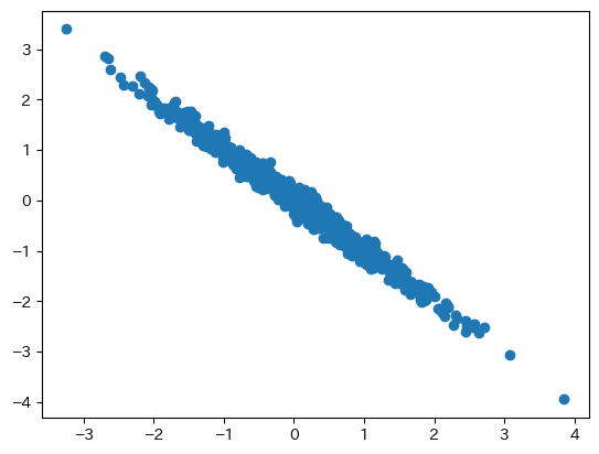
カテゴリカル変数にする前の連続変数に対する推定結果とある程度近い推定値となっていることがわかる

(loadings_cat - loadings).abs().style.set_caption("連続変数の場合との推定値の絶対誤差")

Loading...

# スクリープロットで因子数を探索
eigen = fa.get_eigenvalues()
left = list(range(1, len(eigen[0])+1))
fig, ax = plt.subplots()
ax.plot(left, eigen[0], marker="o")
ax.set(xlabel="因子数（固有値の数）", ylabel="固有値", title="スクリープロット")
ax.axhline(y=1, color="gray", linestyle="--", alpha=0.5)
fig.show()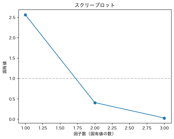

例2：実際のアンケートデータ¶

bfi データ（Big Five Inventory）は、心理学でよく使われる**5因子性格モデル（OCEAN）**に基づいたアンケートデータ

25個の性格項目（各5問 × 5因子）

A1 ～ A5：Agreeableness（協調性）
C1 ～ C5：Conscientiousness（誠実性）
E1 ～ E5：Extraversion（外向性）
N1 ～ N5：Neuroticism（神経症傾向）
O1 ～ O5：Openness（開放性）

import statsmodels.api as sm

# psychパッケージの Big Five Inventory（性格5因子） データ
df = sm.datasets.get_rdataset("bfi", package="psych").data
df.head()

Loading...

from statsmodels.multivariate.factor import Factor
fa = Factor(endog=df.iloc[:, 0:25], n_factor=5, method="ml").fit()
fa.rotate("varimax")
fa.get_loadings_frame()

Loading...

# シンプルにしてみる
df = df.iloc[:, 0:10].dropna()

from statsmodels.multivariate.factor import Factor
fa = Factor(endog=df, n_factor=2, method="ml").fit()
fa.rotate("varimax")
fa.get_loadings_frame()

Loading...

df.corr().style.format("{:.3f}").background_gradient()

Loading...

# 相関係数をとってみる
from ordinalcorr import hetcor
corr = hetcor(df)
corr.style.format("{:.3f}").background_gradient()

Loading...

fa = Factor(corr=corr, n_factor=2, method="ml").fit()
fa.rotate("varimax")
fa.get_loadings_frame()

Loading...

# カテゴリの数を減らしてみる
df_cat = df.copy()
for col in df.columns:
    df_cat[col] = pd.cut(df[col], bins=3, labels=range(3)).astype(int)

# 相関係数をとってみる
from ordinalcorr import hetcor
corr = hetcor(df_cat, n_unique=50)
corr.style.format("{:.3f}").background_gradient()

Loading...

fa = Factor(corr=corr, n_factor=2, method="ml").fit()
fa.rotate("varimax")
fa.get_loadings_frame()

Loading...

参考¶

Hofacker, C. (2004). Exploratory Factor Analysis, Mathematical Marketing. http://www.openaccesstexts.org/pdf/Quant_Chapter_11_efa.pdf
J Bai, K Li (2012). Statistical analysis of factor models of high dimension. Annals of Statistics. https://arxiv.org/pdf/1205.6617.pdf
【Pythonで統計モデル】因子分析4：カテゴリカル因子分析｜福中公輔

ビジネスにおいてはどういったところで応用されるのか？¶

因子分析モデル¶

1因子モデル¶

mmm因子モデル¶

因子分析モデル（行列表現）¶

パラメータの推定¶

Λ,Ψ\mathbf{\Lambda}, \mathbf{\Psi}Λ,Ψの推定（最尤推定法による例）¶

f\mathbf{f}fの推定（バートレット法による例）¶

実装例¶

主成分分析との違い¶

妥当性と信頼性¶

信頼性係数¶

クロンバックのα\alphaα係数¶

Messickの妥当性概念¶

探索的因子分析¶

サンプルデータを生成して因子分析を実行してみる¶

statsmodelsパッケージでの推定¶

factor-analyzerパッケージでの推定¶

scikit-learnの因子分析¶

確認的因子分析¶

カテゴリカル因子分析¶

実装例¶

例2：実際のアンケートデータ¶

参考¶

$m$ 因子モデル¶

$\mathbf{\Lambda}, \mathbf{\Psi}$ の推定（最尤推定法による例）¶

$\mathbf{f}$ の推定（バートレット法による例）¶

クロンバックの $\alpha$ 係数¶