LOWESS

散布図に従う近似線を描くために開発された局所回帰。 LOESS (locally estimated scatterplot smoothing) や LOWESS (locally weighted scatterplot smoothing) と呼ばれる。

import numpy as np
np.random.seed(0)
x = np.linspace(0, 7, 100)
y = np.sin(x) + np.random.normal(0, 0.2, 100)

import statsmodels.api as sm
smoothed = sm.nonparametric.lowess(exog=x, endog=y, frac=0.2, it=3)

import matplotlib.pyplot as plt
fig, ax = plt.subplots()
ax.scatter(x, y)
ax.plot(smoothed[:, 0], smoothed[:, 1], c="k")
ax.set(xlabel="x", ylabel="y")
fig.show()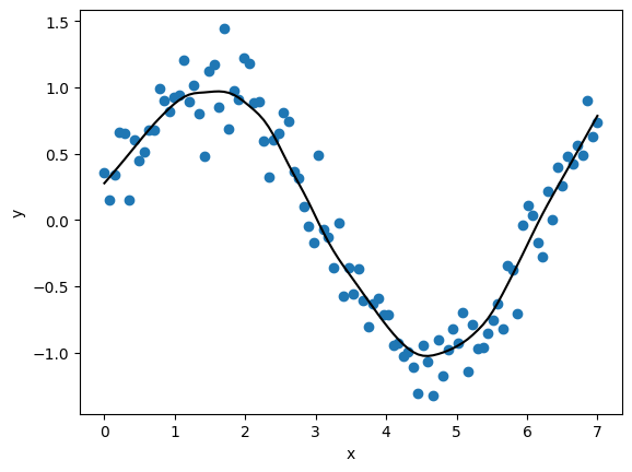

LOWESSのアルゴリズム¶

Cleveland (1979). に記されたアルゴリズムは以下の通り。

$i$ 番目のサンプルの目的変数 $y_i$ を特徴量 $x_i$ とノンパラメトリックの平滑化関数 $g(x_i)$ で近似することを考える。

y_i = g(x_i) + \epsilon_i

(1)

ここで $\epsilon_i$ は平均0で分散が一定の確率変数である。

1. 重みの計算と $r$ 個の最近傍サンプルの取得¶

$x_i$ について、 $j=1,\dots,n$ にわたって $|x_i - x_j|$ で距離を測り、 $r$ 番目に近いサンプルとの距離を $h_i$ とする。

重み関数 $W(\cdot)$ を用いて、 $k=1,\dots,n$ について

w_k(x_i) = W(h_i^{-1}(x_k - x_i))

(2)

を計算する

ここで重み関数 $W(\cdot)$ は以下の性質を満たすものとする

$|x| < 1$ について $W(x) > 0$
$W(-x)=W(x)$
$W(x)$ は $x \geq 0$ について非増加関数
$|x| \geq 1$ について $W(x)=0$

$h_i^{-1}(x_k - x_i)$ は分子の $x_k - x_i$ の絶対値が分母の $h_i$ より大きければ $|h_i^{-1}(x_k - x_i)| \geq 1$ になるので重みが0になる。つまり、サンプルとして回帰に使用されなくなる。なので重み関数は近傍の $r$ 個のサンプルを取り出しつつ、 $r$ 個のサンプルにも距離に応じた重みをかける操作となる。

$W$ の例として tricube functionが考えられる

W(x) = \begin{cases} (1-|x|^3)^3 & \text { for } \quad|x|<1 \\ 0 \quad & \text { for } \quad|x| \geqslant 1 \end{cases}

(3)

def tricube(x: float) -> float:
    if np.abs(x) >= 1:
        return 0
    return (1 - np.abs(x)**3 )**3

x = np.linspace(-2, 2, 100)
w = [tricube(x_i) for x_i in x]

# 別のやり方
# w = (1 - np.abs(x)**3)**3
# w[np.abs(x) >= 1] = 0
fig, ax = plt.subplots(figsize=[4,3])
ax.plot(x, w)
ax.set(title="tricube weight function", xlabel="x", ylabel="W(x)")
fig.show()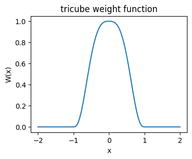

2. 多項式回帰のフィッティング¶

非線形回帰として $d$ 次の多項式回帰を行う

\min_{\beta_0,\dots,\beta_d} ~ \sum_{k=1}^n w_k\left(x_i\right)\left(y_k-\beta_0-\beta_1 x_k-\ldots-\beta_d x_k^d\right)^2

(4)

\hat{y}_i=\sum_{j=0}^d \hat{\beta}_j\left(x_i\right) x_i^j

(5)

3. ロバスト性重み $\delta$ の計算¶

続いて、外れ値の影響を除外するための重みを計算する。 bisquare weight function $B(x)$ を以下のように定義する

B(x) = \begin{cases} (1 - x^2)^2 & \text { for } \quad|x| < 1 \\ 0 \quad & \text { for } \quad|x| \geqslant 1 \end{cases}

(6)

残差 $e_i = y_i - \hat{y}_i$ の絶対値 $|e_i|$ の中央値を $s$ とする。ロバスト性重み（robustness weights）を

\delta_k = B(e_k / 6s)

(7)

と定義する。 $B(x)$ もtricube functionと似た形状であり、残差の絶対値の中央値の6倍（ $6s$ ）以上の絶対値の残差 $|e_k/6s| \geq 1$ を持つ外れ値は重み $\delta_k$ がゼロになり、推定に含まれなくなるので、推定からハズレ値の影響を除外できる。

def bisquare(x: float) -> float:
    if np.abs(x) >= 1:
        return 0
    return (1 - x**2 )**2

x = np.linspace(-2, 2, 100)
b = [bisquare(x_i) for x_i in x]
fig, ax = plt.subplots(figsize=[4,3])
ax.plot(x, b)
ax.set(title="bisquare weight function", xlabel="x", ylabel="B(x)")
fig.show()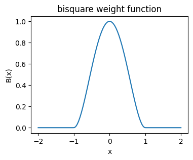

4. $\delta$ で重み付け回帰を行う¶

また $d$ 次多項式回帰を行い、新たな推定値 $\hat{y}_i$ を得る。このとき、重みは $\delta_k w_k (x_i)$ を使う。

5. 繰り返す¶

3.と4.のステップを $t$ 回繰り返す。

実装¶

# サンプルデータ
import numpy as np
n = 100
np.random.seed(0)
x = np.linspace(0, 7, n)
y = np.sin(x) + np.random.normal(0, 0.2, n)

import matplotlib.pyplot as plt
fig, ax = plt.subplots()
ax.scatter(x, y)
ax.set(xlabel="x", ylabel="y")
fig.show()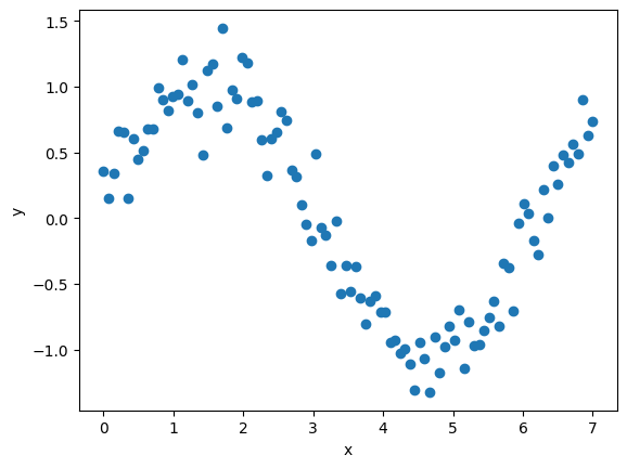

frac = 0.66 # 使用するサンプルの割合
r = int(frac * n)  # 使用する近傍のサンプル数
d = 3  # 多項式回帰の次数
t = 3  # iteration

def tricube(x: np.array) -> np.array:
    w = (1 - np.abs(x)**3)**3
    w[np.abs(x) >= 1] = 0
    return w

def bisquare(x: np.array) -> np.array:
    w = (1 - np.abs(x)**2)**2
    w[np.abs(x) >= 1] = 0
    return w

# d次多項式を作るための特徴量生成
X = np.vstack([x**j for j in range(d)]).T

n = X.shape[0]
delta = np.ones_like(x)
y_pred = np.zeros_like(x)
for _ in range(t):
    for i in range(n):
        # 重みの計算
        dist = x - x[i]
        idx = np.argsort(np.abs(dist))[:r]
        h_i = np.abs(dist[idx]).max() # r番目に近いdiff
        w = tricube(dist / h_i)
        W = np.diag(delta * w)
    
        # WLS
        beta = np.linalg.inv(X.T @ W @ X) @ X.T @ W @ y
        y_pred[i] = X[i,:] @ beta
    
    e = y - y_pred
    s = np.median(np.abs(e))
    delta = bisquare(e / (6 * s))

import matplotlib.pyplot as plt
fig, ax = plt.subplots()
ax.scatter(x, y)
ax.plot(x, y_pred, c="k")
ax.set(xlabel="x", ylabel="y")
fig.show()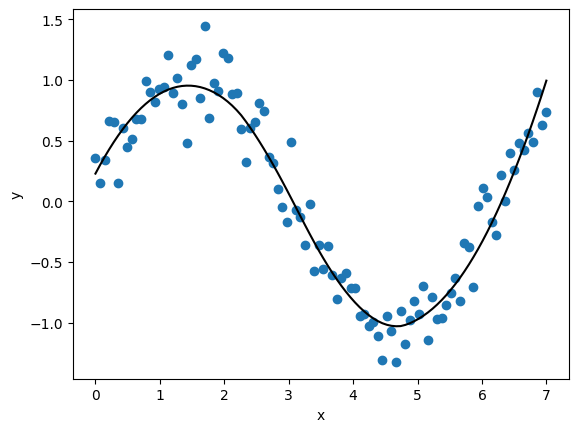

最近のLOWESSアルゴリズム¶

Wikipediaには、重み関数がtricubeではなくGaussianを使うものが紹介されている

Gaussian weight functionとは、2つのデータ点の特徴量ベクトル $x, x' \in \mathbb{R}^m$ （ $m$ は特徴量の次元数）について、

w(x, x', \alpha)=\exp \left(-\frac{\|x-x'\|^2}{2 \alpha^2}\right)

(8)

といったもの。

参考¶

Local regression - Wikipedia
Cleveland, W. S. (1979). Robust locally weighted regression and smoothing scatterplots. Journal of the American statistical association, 74(368), 829-836.