証明
残差への回帰は
であり、
を代入するとそれぞれ
となる。
これらをそれぞれ被説明変数、説明変数として最小二乗推定すると
(は冪等で対称な行列のため2行目で計算が簡略化できている)
次に、すべての説明変数をに回帰したとき
のの係数の推定量を求める。二乗誤差の最小化の解
の1階の条件は
となる。を消すためには、2つ目の式に左からを掛けて
これを第1式に足すと
となる。
これを変形すると
となり、残差回帰の解と一致する。
数値例
import numpy as np

n = 100
d = 4
k = 1
np.random.seed(0)
beta = np.array(list(range(1, d + 1)))
print(f"{beta=}")
X = np.random.uniform(size=(n, d))
e = np.random.normal(size=n) * 0.1
Y = X @ beta + e

X1 = X[:, :k]
X2 = X[:, k:]
beta1 = beta[:k]
beta2 = beta[k:]
assert np.allclose(Y, X1 @ beta1 + X2 @ beta2 + e)
beta=array([1, 2, 3, 4])
# I - X_2 (X_2^T X_2)^{-1} X_2^T は冪等で対称な行列
I = np.eye(n)
M = (I - X2 @ np.linalg.inv(X2.T @ X2) @ X2.T)
assert np.allclose(M.T, M)
assert np.allclose(M, M @ M)
delta = np.linalg.inv(X2.T @ X2) @ X2.T @ X1
gamma = np.linalg.inv(X2.T @ X2) @ X2.T @ Y
Y_tilde = (Y - X2 @ gamma)
X_tilde = (X1 - X2 @ delta)
# 残差回帰
beta_hat2 = np.linalg.inv(X_tilde.T @ X_tilde) @ X_tilde.T @ Y_tilde
beta_hat2.round(1)array([1.])# 通常の線形回帰
beta_hat1 = np.linalg.inv(X.T @ X) @ X.T @ Y
beta_hat1.round(1)array([1. , 2. , 2.9, 4. ])残差の作図
Source
import matplotlib.pyplot as plt
import japanize_matplotlib

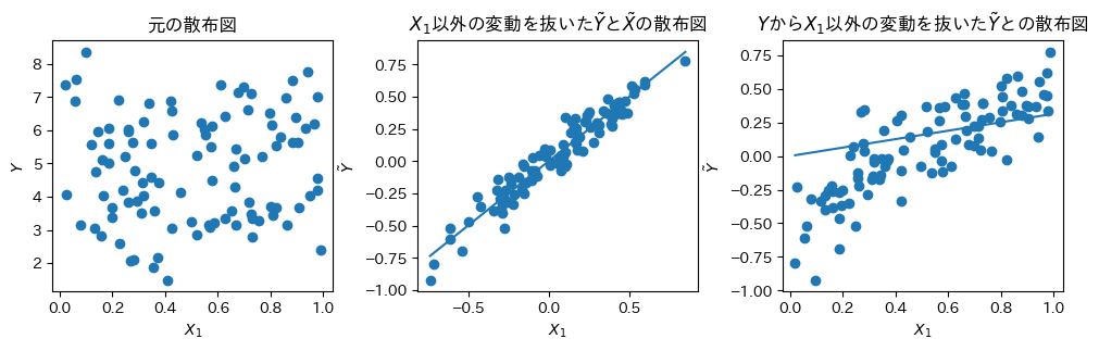
fig, axes = plt.subplots(figsize=[12, 3], ncols=3)
fig.subplots_adjust(wspace=0.3)
axes[0].scatter(X1, Y)
axes[0].set(ylabel=r"$Y$", xlabel=r"$X_1$", title="元の散布図")

axes[1].scatter(X_tilde, Y_tilde)
axes[1].set(ylabel=r"$\tilde{Y}$", xlabel=r"$X_1$", title=r"$X_1$以外の変動を抜いた$\tilde{Y}$と$\tilde{X}$の散布図")

beta_ = np.linalg.inv(X_tilde.T @ X_tilde) @ X_tilde.T @ Y_tilde
xrange = np.linspace(X_tilde.min(), X_tilde.max(), 100)
axes[1].plot(xrange, xrange.reshape(-1, 1) @ beta_)

axes[2].scatter(X1, Y_tilde)
axes[2].set(ylabel=r"$\tilde{Y}$", xlabel=r"$X_1$", title=r"$Y$から$X_1$以外の変動を抜いた$\tilde{Y}$との散布図")
beta_ = np.linalg.inv(X1.T @ X1) @ X1.T @ Y_tilde
xrange = np.linspace(X1.min(), X1.max(), 100)
axes[2].plot(xrange, xrange.reshape(-1, 1) @ beta_)

fig.show()
/tmp/ipykernel_88307/1189295102.py:22: UserWarning: Matplotlib is currently using module://matplotlib_inline.backend_inline, which is a non-GUI backend, so cannot show the figure.
fig.show()
外生性・直交条件からの説明
浅野・中村では誤差が直交することから証明するスタイルで、有斐閣の本はより直接的に証明している
数値例
import numpy as np

n = 1000
np.random.seed(0)
x0 = np.ones(shape=(n, ))
x2 = np.random.uniform(0, 1, size=n)
x1 = 3 * x2 + np.random.uniform(0, 1, size=n) + np.random.normal(0, 1, size=n)
X = np.array([ x0, x1, x2 ]).T
e = np.random.normal(0, 1, size=n)

beta = np.array([10, 5, 7])  # 真のbeta
y = X @ beta + e
np.corrcoef(X, rowvar=False)/home/mitama/notes/.venv/lib/python3.10/site-packages/numpy/lib/function_base.py:2897: RuntimeWarning: invalid value encountered in divide
c /= stddev[:, None]
/home/mitama/notes/.venv/lib/python3.10/site-packages/numpy/lib/function_base.py:2898: RuntimeWarning: invalid value encountered in divide
c /= stddev[None, :]
array([[       nan,        nan,        nan],
       [       nan, 1.        , 0.64601675],
       [       nan, 0.64601675, 1.        ]])
class OLS:
def fit(self, X, y):
self.beta_ = np.linalg.inv(X.T @ X) @ X.T @ y
return self
def predict(self, X):
return X @ self.beta_1. をに回帰する
# 1. 𝑦 を 𝑥1 に回帰する
OLS().fit(X, y).beta_array([9.98226817, 5.03640436, 6.80111723])2. をに回帰する
ここではをに回帰した残差
# 2. 𝑦 を 𝑥̃ 1 に回帰する
X_ = X[:, [0, 2]] # x0, x2だけのX
x1_res = x1 - OLS().fit(X_, x1).predict(X_)
# 切片を付けた場合
X_ = np.array([ x0, x1_res ]).T
OLS().fit(X_, y).beta_array([23.29878836, 5.03640436])# 切片を付けない場合
OLS().fit(x1_res.reshape(-1, 1), y).beta_array([5.03640436])3. をに回帰する
ここではをに回帰した残差
# 3. 𝑦̃ を 𝑥̃ 1 に回帰する
X_ = X[:, [0, 2]] # x0, x2だけのX
y_res = y - OLS().fit(X_, y).predict(X_)
# 切片を付けない場合
OLS().fit(x1_res.reshape(-1, 1), y_res).beta_array([5.03640436])# 切片を付けた場合
X_ = np.array([ x0, x1_res ]).T
OLS().fit(X_, y_res).beta_array([4.27435864e-15, 5.03640436e+00])partialling out
OLS推定では説明変数と残差の共分散はゼロになる。
というモデルがあったとき、説明変数を他のすべての説明変数に回帰すると、その残差は説明変数の分散の情報を残す一方で他の説明変数とは無相関になる。
したがってをこの残差に回帰すると、その回帰係数はに対するの影響のみを示す。
→他の変数の影響を排除(partialling out)できる
statsmodelsで簡単に実行できる
statsmodelsのplot_regress_exog関数は残差の分析に関する4つの図をまとめて出力でき、そのうちのひとつ「Partial regression plot」がpartialling outした残差同士の散布図になっている。
import statsmodels.api as sm
results = sm.OLS(y, X).fit()
fig = sm.graphics.plot_regress_exog(results, 'x2')Source
import matplotlib.lines as mlines
import matplotlib.collections as mcoll
def change_alpha(fig, alpha = 0.2):
"""plot_regress_exogの透明度を変える"""
for ax in fig.axes:
# scatter() の点(0番だけ)
for coll in ax.collections:
if isinstance(coll, mcoll.PathCollection):
coll.set_alpha(alpha)
# plot(..., marker='o', linestyle='None') の点(1〜3番)
for line in ax.lines:
if isinstance(line, mlines.Line2D):
has_marker = line.get_marker() not in (None, "", "None")
no_line = line.get_linestyle() in ("None", " ", "", None)
if has_marker and no_line:
line.set_alpha(alpha)
import statsmodels.api as sm
results = sm.OLS(y, X).fit()
fig = sm.graphics.plot_regress_exog(results, 'x2')
change_alpha(fig, alpha = 0.2)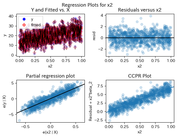
統計的因果推論
Belloni et al. (2014)のpost-double selection
Chernozhukov et al. (2018)のDouble/debiased machine learning (DML)
などで用いられる。DMLはモデルの学習アルゴリズムに機械学習を許容するので、過学習や正則化によるバイアスに対処するためのcross-fittingという推定方法を提案している。
歴史:Yule-Frisch-Waugh-Lovell Theorem
[2307.00369] The Yule-Frisch-Waugh-Lovell Theorem
FWLの前にYuleがいたらしい
通常、Frisch and Waugh (1933) と Lovell (1963) の名前をとって Frisch-Waugh-Lovell Theoremと呼ぶ。しかしこの論文によれば Yule (1907) も重要な貢献をしており、計量経済学では知名度がないものの統計学分野では注目されているため、FWL定理ではなくYFWL定理と呼ぶことを提案している。
参考文献
FWL
Frisch, R., & Waugh, F. V. (1933). Partial time regressions as compared with individual trends. Econometrica: Journal of the Econometric Society, 387-401.
Lovell, M. C. (1963). Seasonal adjustment of economic time series and multiple regression analysis. Journal of the American Statistical Association, 58(304), 993-1010.
import numpy as np
# データを生成
n = 1000
np.random.seed(0)
x0 = np.ones(shape=(n, ))
x2 = np.random.uniform(0, 1, size=n)
x3 = np.random.uniform(0, 1, size=n)
x1 = x2 + x3 + np.random.normal(0, 1, size=n)
X = np.array([ x0, x1, x2, x3 ]).T
e = np.random.normal(0, 1, size=n)
beta = np.array([10, 5, 7, 3]) # 真のbeta
y = X @ beta + e
class OLS:
    def fit(self, X, y):
        self.beta_ = np.linalg.inv(X.T @ X) @ X.T @ y
        return self

    def predict(self, X):
        return X @ self.beta_
1. をに回帰する
# 1. 𝑦 を 𝑥1 に回帰する
OLS().fit(X, y).beta_array([9.95538609, 5.03200117, 6.87766976, 3.05740035])# 2. 𝑦 を 𝑥̃ 1 に回帰する
X_ = X[:, [0, 2, 3]]
x1_res = x1 - OLS().fit(X_, x1).predict(X_)
# 切片を付けない場合
OLS().fit(x1_res.reshape(-1, 1), y).beta_array([5.03200117])import matplotlib.pyplot as plt
plt.scatter(x1_res, x1)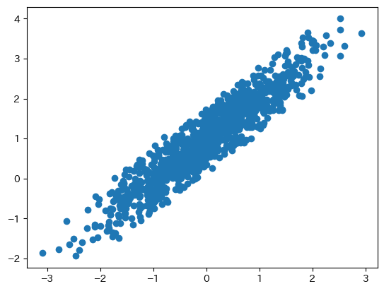
from scipy.stats import pearsonr
pearsonr(x1_res, x1).statistic.round(3)0.933説明変数1つずつでpartialling outできないか?
for all nuisance parameter indices
# 2. 𝑦 を 𝑥̃ 1 に回帰する
x1_res = x1.copy()
nuisance_indices = [0, 2, 3]
for i in nuisance_indices:
    X_ = X[:, [i]]
    x1_res = x1_res - OLS().fit(X_, x1_res).predict(X_)
    print(f"corr(x1_res, x1): {pearsonr(x1_res, x1).statistic:.3f}")
    print(f"beta1           : {OLS().fit(x1_res.reshape(-1, 1), y).beta_[0]:.3f}")

OLS().fit(x1_res.reshape(-1, 1), y).beta_
corr(x1_res, x1): 1.000
beta1 : 5.750
corr(x1_res, x1): 0.998
beta1 : 3.435
corr(x1_res, x1): 0.998
beta1 : 2.925
array([2.92542108])# 2. 𝑦 を 𝑥̃ 1 に回帰する
x1_res = x1.copy()
nuisance_indices = [0, 2, 3]
for i in nuisance_indices[::-1]:
X_ = X[:, [i]]
x1_res = x1_res - OLS().fit(X_, x1_res).predict(X_)
print(f"corr(x1_res, x1): {pearsonr(x1_res, x1).statistic:.3f}")
print(f"beta1 : {OLS().fit(x1_res.reshape(-1, 1), y).beta_[0]:.3f}")
OLS().fit(x1_res.reshape(-1, 1), y).beta_corr(x1_res, x1): 0.887
beta1 : 7.193
corr(x1_res, x1): 0.876
beta1 : 2.998
corr(x1_res, x1): 0.876
beta1 : 4.613
array([4.61310126])- Lovell, M. C. (1963). Seasonal Adjustment of Economic Time Series and Multiple Regression Analysis. Journal of the American Statistical Association, 58(304), 993–1010. 10.1080/01621459.1963.10480682