目的変数や説明変数を対数変換すると、推定結果の解釈が変わる
| モデル | 係数の解釈 |
|---|---|
| 「が1単位増加すると、が単位増加する」 | |
| 「が1%増加すると、が単位増加する」 | |
| 「が1単位増加すると、が%増加する」 | |
| 「が1%増加すると、が%増加する」 |
次のようなデータを使って実際にモデルをあてはめつつ確認していく
Source
import numpy as np
import pandas as pd
import matplotlib.pyplot as plt
import seaborn as sns
import statsmodels.api as sm
import statsmodels.formula.api as smf


# 真のデータ生成過程
n = 100
np.random.seed(0)
x = np.random.uniform(1, 100, size=n)
x = np.sort(x)
e = np.random.normal(loc=0, scale=15, size=n)
beta0 = 100
beta1 = 3
y = beta0 + beta1 * x + e

df = pd.DataFrame({"y": y, "x": x})
plt.scatter(x, y)
plt.xlabel("x")
plt.ylabel("y")
plt.title(f"y = {beta0} + {beta1} * x + e")
plt.show()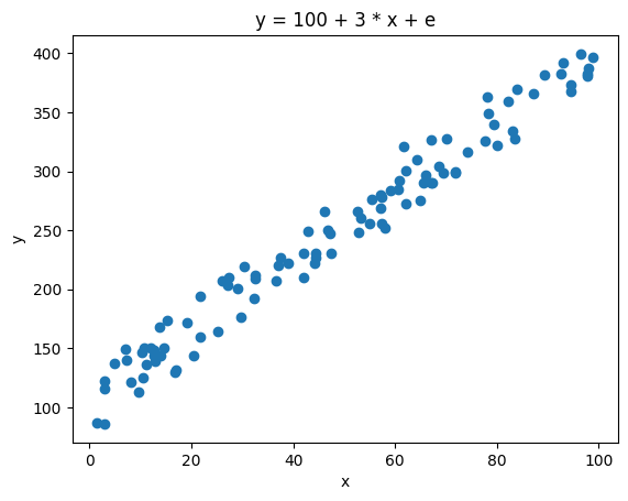
Source
model = smf.ols('y ~ x', data=df).fit()
beta = model.params.to_list()

y_pred = model.predict(df[["x"]])

fig, ax = plt.subplots()
ax.scatter(x, y)
ax.set(xlabel="x", ylabel="y", title="y = β0 + β1 x")
ax.plot(x, y_pred, label=f"estimated model: y = {beta[0]:.1f} + {beta[1]:.2f} x")
ax.legend()
fig.show()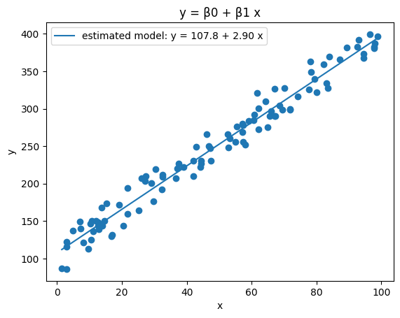
について
はテイラー近似から導出される。まずテイラー近似について述べる
とおくと、その次の微分は
となる。もしなら
となる。
これをでのテイラー展開(つまりマクローリン展開)
にあてはめると、
となる。これはが極めて小さな値()であればやといった値は非常に小さくなるため、となる。
よってとなる
数値計算的に確かめると、以下のようになる
import numpy as np
x = 0.01
print(f"log: {np.log(1 + x):.7f}")
print(f"approx 1: {x:.7f}")
print(f"approx 2: {x - (x**2 / 2):.7f}")
print(f"approx 3: {x - (x**2 / 2) + (x**3 / 3):.7f}")
log: 0.0099503
approx 1: 0.0100000
approx 2: 0.0099500
approx 3: 0.0099503Source
model = smf.ols('y ~ np.log(x)', data=df).fit()
beta = model.params.to_list()
y_pred = model.predict(df[["x"]])

fig, axes = plt.subplots(ncols=2, figsize=[12, 4])
axes[0].scatter(x, y)
axes[0].set(xlabel="x", ylabel="y", title="y = β0 + β1 log(x)")
axes[0].plot(x, y_pred, label=f"estimated model: y = {beta[0]:.1f} + {beta[1]:.3g} log(x)")
axes[0].legend()

axes[1].scatter(np.log(x), y)
axes[1].set(xlabel="log(x)", ylabel="y", title="y = β0 + β1 log(x)")
axes[1].plot(np.log(x), y_pred, label=f"estimated model: y = {beta[0]:.1f} + {beta[1]:.3g} log(x)")
axes[1].legend()

fig.show()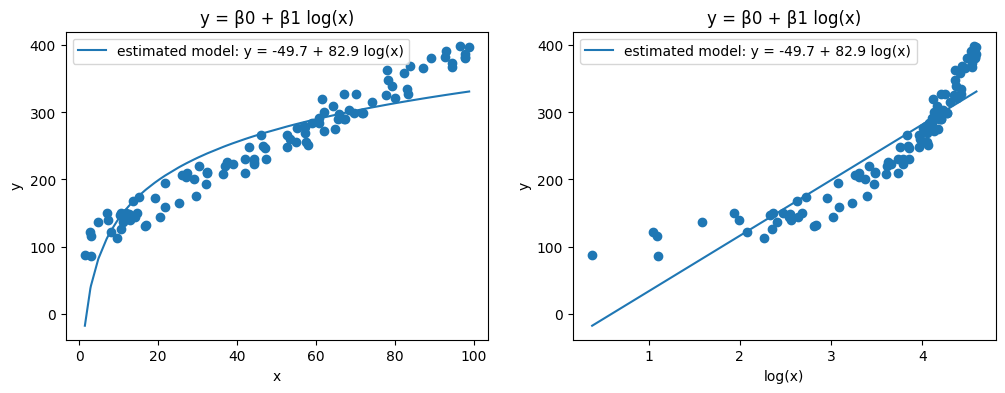
np.log(1.01)0.009950330853168092x0 = 50
y1 = beta[0] + beta[1] * np.log(x0)
y2 = beta[0] + beta[1] * np.log(x0 * 1.01)
print(f"xが1%増加したときのyの増分 = {y2 - y1:.3f}")xが1%増加したときのyの増分 = 0.825
の近似誤差が多少あるが、おおむね「が1%増加すると、が単位増加する」という関係になる。
について
とおくと、その次の微分は
となる。もしなら
となる。
これをでのテイラー展開(つまりマクローリン展開)
にあてはめると、
となる。
が極めて小さな値()であればやといった値は非常に小さくなるため、となる。
よってとなる
数値計算的に確かめると、以下のようになる
import numpy as np
x = 0.1
print(f"""
x         : {x}
exp(x) - 1: {np.exp(x) - 1:.7f}

マクローリン近似
もとの値  exp(x)             = {np.exp(x):.7f}
1次近似   1 + x              = {1 + x:.7f}
2次近似   1 + x + (x^2 / 2!) = {1 + x + (x**2 / (1 * 2)):.7f}
""")
x : 0.1
exp(x) - 1: 0.1051709
マクローリン近似
もとの値 exp(x) = 1.1051709
1次近似 1 + x = 1.1000000
2次近似 1 + x + (x^2 / 2!) = 1.1050000Source
model = smf.ols('np.log(y) ~ x', data=df).fit()
beta = model.params.to_list()
y_pred = model.predict(df[["x"]])

fig, axes = plt.subplots(ncols=2, figsize=[12, 4])

axes[0].scatter(x, y)
axes[0].set(xlabel="x", ylabel="y, exp(y_hat)", title="y = β0 + β1 x")
axes[0].plot(x, np.exp(y_pred), label=f"estimated model: log(y) = {beta[0]:.1f} + {beta[1]:.2g} x")
axes[0].legend()

axes[1].scatter(x, np.log(y))
axes[1].set(xlabel="x", ylabel="log(y), y_hat", title="log(y) = β0 + β1 x")
axes[1].plot(x, y_pred, label=f"estimated model: log(y) = {beta[0]:.1f} + {beta[1]:.2g} x")
axes[1].legend()

fig.show()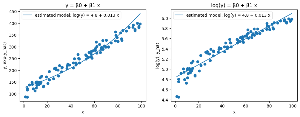
x0 = 50
y1 = beta[0] + beta[1] * x0
y2 = beta[0] + beta[1] * (x0 + 1)
print(f"xが1単位増加したときのyの増分 = {y2 - y1:.3f}")
xが1単位増加したときのyの増分 = 0.013
(4) 
「が1%増加すると、が%増加する」
Source
model = smf.ols('np.log(y) ~ np.log(x)', data=df).fit()
beta = model.params.to_list()
y_pred = model.predict(df[["x"]])

fig, axes = plt.subplots(ncols=2, figsize=[12, 4])

axes[0].scatter(x, y)
axes[0].set(xlabel="x", ylabel="y, exp(y_hat)", title="log(y) = β0 + β1 log(x)")
axes[0].plot(x, np.exp(y_pred), label=f"estimated model: log(y) = {beta[0]:.1f} + {beta[1]:.2g} log(x)")
axes[0].legend()

axes[1].scatter(np.log(x), np.log(y))
axes[1].set(xlabel="log(x)", ylabel="log(y), y_hat", title="log(y) = β0 + β1 log(x)")
axes[1].plot(np.log(x), y_pred, label=f"estimated model: log(y) = {beta[0]:.1f} + {beta[1]:.2g} log(x)")
axes[1].legend()

fig.show()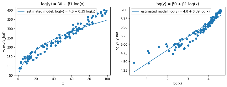
x0 = 50
y1 = beta[0] + beta[1] * np.log(x0)
y2 = beta[0] + beta[1] * np.log(x0 + 1)
print(f"xが1%増加したときのyの増分 = {y2 - y1:.3f}")
xが1%増加したときのyの増分 = 0.008
y1 = model.predict(pd.DataFrame([{"x": x0}])).to_numpy()[0]
y2 = model.predict(pd.DataFrame([{"x": x0 + 1}])).to_numpy()[0]
print(f"xが1単位増加したときのyの増分 = {y2 - y1:.3f}")
xが1単位増加したときのyの増分 = 0.008
別データ例:賃金データ
RのAERパッケージに含まれるCPS1985という1985年の賃金のデータを例に取る。教育年数が1年ふえるごとに賃金は何%増えるのだろうか。
Source
import statsmodels.api as sm
cps = sm.datasets.get_rdataset("CPS1985", "AER").data.assign(log_wage = np.log(cps["wage"]))

fig, axes = plt.subplots(ncols=2, figsize=[8, 4])

reg = smf.ols('wage ~ education', data=cps).fit()
axes[0].scatter(cps["education"], cps["wage"], color="black", alpha=0.5
)axes[0].set(xlabel="education", ylabel="wage")
axes[0].plot(cps["education"], reg.predict(cps),
             label=f"wage = {reg.params['Intercept']:.3f} + {reg.params['education']:.3f} education")
axes[0].legend()


reg = smf.ols('log_wage ~ education', data=cps).fit()
axes[1].scatter(cps["education"], cps["log_wage"], color="black", alpha=0.5)
axes[1].set(xlabel="education", ylabel="log_wage")
axes[1].plot(cps["education"], reg.predict(cps),
             label=f"log_wage = {reg.params['Intercept']:.3f} + {reg.params['education']:.3f} education")
axes[1].legend()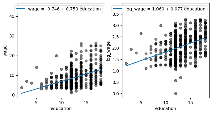
モデルに投入するeducationの値が1上がるごとに、概ね0.079 = 7.9%程度上がる
reg = smf.ols('log_wage ~ education', data=cps).fit()
test = pd.DataFrame({"education": range(21)})
test["log_wage_pred"] = reg.predict(test)  # 予測値を入れる
test["wage_pred"] = np.exp(test["log_wage_pred"])
test["wage_pred_diff"] = test["wage_pred"].diff()
test["wage_pred_change"] = test["wage_pred"].pct_change()
test["log_wage_pred_change"] = test["log_wage_pred"].pct_change()
test.head(10)
Loading...
最近は逆双曲線変換をするらしい
長所:
対数と同様に振る舞う:被説明変数と説明変数両方にarsinh()している場合推定した回帰係数が弾力性になる(xとyが10以上などある程度大きい値のとき)
値がゼロの観測値を維持する:
値が負の観測値も維持する(があるため)
短所:
推定した係数が弾力性になるにはxとyが10以上などある程度大きい値のときのみ → 零や負の値を使えるという利点があまり活きない