概要
LightGBMのような最近のGBDTで使われている決定木では、葉の出力は誤差関数の2次のテイラー近似をもとに、以下のように計算される(このあたりはChen & Guestrin, 2016が比較的わかりやすい)
ここでは誤差関数の勾配、は誤差関数の二次の微分である。
このを32bitや64bitのfloatではなく、4bitなどの低ビット幅の整数で保持しよう、というのが量子化である。
現代的なGBDTの学習の流れ
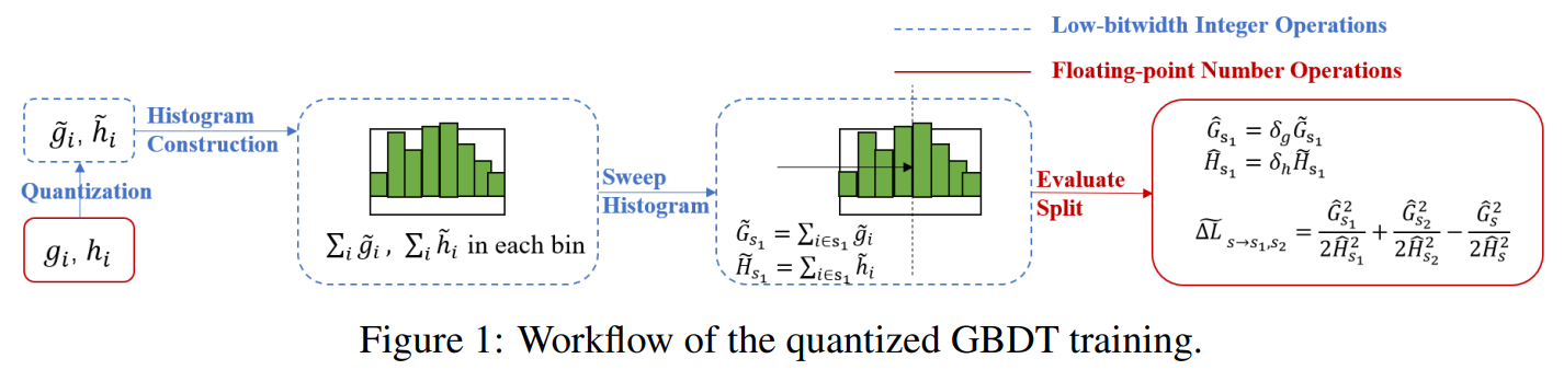
(Shi et al. (2022). Quantized training of gradient boosting decision trees.より)
まず、GBDTの学習の流れを再確認し、notationを決める
勾配ブースティング決定木(GBDT)は複数の決定木を組み合わせるアンサンブル学習のアプローチをとる。
各iterationでは現状の予測値に基づくGradientとHessianを計算し、負の勾配を近似するように決定木を学習する。
回目の反復において、現状のサンプルの予測値をとすると、誤差関数のgradientとhessianは
となる。
葉について、葉に含まれるデータの番号(index)の集合をとする。葉におけるとのサンプルについての合計を
と表記することにすると、反復回目において木構造が固定された下で、訓練誤差は二次のテイラー近似により
と表すことができる。
ここでは定数で、は葉の予測値である。近似誤差の最小化により最適値が得られる
最適な木構造を探すのは困難であるため、木は貪欲かつ反復的に訓練される。
葉を2つの子に分割するとき、近似損失の減少分は次のように計算できる。
葉にとっての最適な分割条件の探索は、すべての特徴のすべての分割候補点を数え上げて、最も損失の減少が多いものが選ばれる。
LightGBMでは最適分割点の探索を高速化するためにヒストグラムを使う。histogram based GBDTの基本的なアイデアは特徴量の値をbinsに分割する。histogramのbinsは、そのbinに含まれるデータのgradientsとhessiansの総和が記録されている。binsの境界値のみが分割候補点になる。
Algorithm 1 Histogram Construction for Leaf
Input: Gradients , Hessians
Input: Bin data data , Data indices in leaf denoted by
Output: Histogram
for do
bin
bin
end for
伝統的にはとには32-bitの浮動小数点数が使われ、histogramへの累計には32-bitか64-bitの浮動小数点数が必要になる。
Framework for Quantized Training
まずとを低ビット幅(low-bitwidth)の整数に量子化する。
すべての訓練サンプルのとのレンジを、等しい長さの区間へと分割する。-bit 整数の勾配を使うために、個の区間を使う。各区間の最後は整数値と対応するため、全体で個の整数値になる。
1次の導関数は正の値も負の値もとるため、半分の区間は負の値のために割り当てられ、残り半分は正の値に割り当てられる。
2次の導関数は一般的にGBDTで使われる誤差関数のほとんどすべてが非負の値をもつため、以下の議論ではと仮定する。
それゆえ、区間の長さはそれぞれに対して
となる。これにより、低ビット幅の勾配は
で計算できる。ここでは浮動小数点数を定数に丸める関数である。
なお、もしが定数なら、量子化する必要はない。
詳細なrounding strategyは4.2節に書く。
Algorithm 1のをに置き換える。もとの勾配の和の計算は整数の和の計算に置き換えられ、histogram binsの統計量とは整数になる。
B = 2
g = [0.1, 0.2, 0.3, 0.4, 0.5, 0.6, 0.7, 0.8, 0.9, 1.0]
delta_g = max([abs(gi) for gi in g]) / (2**(B-1) - 1)
tilde_g = [round(gi / delta_g) for gi in g]
tilde_g
[0, 0, 0, 0, 0, 1, 1, 1, 1, 1]分岐による損失の減少分
のは整数のに置き換えられる。
我々は2から4bitの量子化された勾配が十分よい精度をもたらすことを発見した。また、6.1節と7.4.3節で議論するが、ヒストグラムにおける累積した低ビット幅の勾配には16bit整数で十分であった。それゆえ、大部分の演算は低ビット幅の整数によって行われる。浮動小数点数の演算が必要になるのは本来の勾配とヘシアンとsplit gainを計算するときだけである。とくに、split gainは
と推定される。ここで勾配の統計量のスケールはとを乗じることで復元される。
Figure 1は量子化されたGBDTのワークフローを要約している。
Rounding Strategies and Leaf-Value Refitting
最も近い整数への丸め込み(round-to-nearest)
では精度が大幅に低下することがわかった。
代わりに、 確率的な丸め込み(stochastic rounding)
を用いる(はwith probabilityの意味)。 確率的な丸め込みではであるような値がランダムな値かをとる。
split gainは勾配の総和で計算されるため、確率的な丸め込みは総和への不偏推定量となる。すなわち
である。
確率的な丸め込みの重要性はニューラルネットの量子化学習[13]とDimBoost[16]のヒストグラム分解でも認識されている。
量子化された勾配により、最適なleaf valueは
となり、多くのケースでは良い結果をもたらすのに十分である。
しかし、ランキングなど一部の損失関数では、木の成長が止まったあとに元の勾配でleaf valueをrefittingする方法が精度を向上させることがわかった。BitBoost [8] も同様の方法をとっているが、BitBoostと違い、本手法はsplit gainのヘシアンを木の成長中も考慮するがBitBoostではヘシアンを定数として扱い真のヘシアンをleaf valueのrefittingのときだけ使う。
import pandas as pd
import numpy as np
import matplotlib.pyplot as plt


def stochastic_round(x: float) -> int:
    f = np.floor(x)
    c = np.ceil(x)
    return np.random.choice([f, c], p=[c - x, x - f])

np.random.seed(0)
e = 0.001
x = np.linspace(e, 1-e, 1000)
y = [stochastic_round(xi) for xi in x]


x_c = pd.cut(x, bins=10)

def mid_value(cat):
    return cat.left + ((cat.right - cat.left) / 2)

cat_to_mid = {cat: mid_value(cat) for cat in x_c.categories}

df = pd.DataFrame({
    "x": x,
    "y": y,
    "x_c": x_c.map(cat_to_mid, na_action=None)
})
agg = df.groupby("x_c", observed=True)["y"].agg(["mean", "std"]).reset_index()

fig, ax = plt.subplots()
ax.scatter(x, y, alpha=0.1, label="StochasticRound(x)", edgecolors="steelblue")
ax.errorbar(agg["x_c"], agg["mean"], yerr=agg["std"], alpha=0.9,
            fmt="o", color="gray", label="mean & std of StochasticRound(x)")
            # xerr=(x.max() - x.min()) / 10 / 2,

# for cat in x_c.categories:
#     ax.axvline(cat.left, alpha=0.5, linestyle="--", color="gray")
# ax.axvline(cat.right, alpha=0.5, linestyle="--", color="gray")

ax.set(
    xlabel="x",
    ylabel="StochasticRound(x)",
    title="",
)
ax.legend()
fig.show()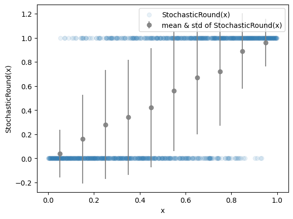
確率的な丸め込みによる
確率的な丸め込みにより、「split gain推定の誤差は高い確率で小さい値に制限される」というsection 5の定理が提供できる。
実験:量子化の有無による差を比較
import lightgbm as lgb
print(f"{lgb.__version__=}")


def gen_dataset(seed=0):
    from sklearn.datasets import make_regression
    X, y = make_regression(n_samples=5_000, n_features=10, noise=0.5, random_state=seed)

    from sklearn.model_selection import train_test_split
    X_train, X_test, y_train, y_test = train_test_split(X, y, train_size=0.8, random_state=0)
    X_train, X_val, y_train, y_val = train_test_split(X_train, y_train, train_size=0.8, random_state=0)

    import lightgbm as lgb
    lgb_train = lgb.Dataset(X_train, y_train)
    lgb_val = lgb.Dataset(X_val, y_val, reference=lgb_train)
    return lgb_train, lgb_val, X_test, y_test


def train(params, lgb_train, lgb_val):
    logs = {}
    model = lgb.train(
        params,
        lgb_train,
        num_boost_round=100_000,
        valid_sets=[lgb_train, lgb_val],
        callbacks=[
            lgb.early_stopping(stopping_rounds=100),
            lgb.log_evaluation(period=100000),
            lgb.record_evaluation(logs)
        ]
    )
    return model, logs


from tqdm import tqdm
from time import time
from pathlib import Path
from sklearn.metrics import root_mean_squared_error
import joblib
import pandas as pd


def get_model_size(model):
    model_path = Path("model.joblib")
    with open(model_path, "wb") as f:
        joblib.dump(model, f)

    size_mb = model_path.stat().st_size / 1024**2
    model_path.unlink()
    return size_mb


def trials(name, params, n_trials=10):
    train_times = []
    pred_times = []
    rmses = []
    model_sizes = []
    for i in tqdm(range(n_trials)):
        lgb_train, lgb_val, X_test, y_test = gen_dataset(seed=i)

        t0 = time()
        model, _logs = train(params, lgb_train, lgb_val)
        t1 = time()
        train_times.append(t1 - t0)

        t0 = time()
        y_pred = model.predict(X_test)
        t1 = time()
        pred_times.append(t1 - t0)

        rmse = root_mean_squared_error(y_test, y_pred)
        rmses.append(rmse)

        size = get_model_size(model)
        model_sizes.append(size)
    result = pd.DataFrame({
        "Training time": train_times,
        "Inference time": pred_times,
        "RMSE": rmses,
        "Model Size (MB)": model_sizes
    })
    result["条件"] = name
    return result


import os
print(f"{os.cpu_count()=}")
n_trials = 10
results = []

params = {
    'device_type': 'cpu',
    'num_threads': os.cpu_count(),
    'objective': 'mse',
    'metric': 'rmse',
    'num_leaves': 31,
    'learning_rate': 0.1,
    'feature_fraction': 0.8,
    'verbose': -1,
    'seed': 0,
    'deterministic': True,
}

# 量子化なし
result = trials(name="量子化なし", params=params, n_trials=n_trials)
results.append(result)

# 量子化あり
params["use_quantized_grad"] = True
params["num_grad_quant_bins"] = 4

params["quant_train_renew_leaf"] = False
result = trials(name="量子化あり・Renewなし", params=params, n_trials=n_trials)
results.append(result)

params["quant_train_renew_leaf"] = True
result = trials(name="量子化あり・Renewあり", params=params, n_trials=n_trials)
results.append(result)
Output
lgb.__version__='4.3.0'
os.cpu_count()=16
0%| | 0/10 [00:00<?, ?it/s]Training until validation scores don't improve for 100 rounds
10%|█ | 1/10 [01:41<15:12, 101.39s/it]Early stopping, best iteration is:
[1781] training's rmse: 0.115047 valid_1's rmse: 41.0182
Training until validation scores don't improve for 100 rounds
Early stopping, best iteration is:
[1650] training's rmse: 0.0972269 valid_1's rmse: 27.826
20%|██ | 2/10 [04:43<19:51, 148.95s/it]Training until validation scores don't improve for 100 rounds
Early stopping, best iteration is:
[3078] training's rmse: 0.00376388 valid_1's rmse: 46.6675
30%|███ | 3/10 [08:14<20:40, 177.28s/it]Training until validation scores don't improve for 100 rounds
40%|████ | 4/10 [08:22<11:02, 110.36s/it]Early stopping, best iteration is:
[1642] training's rmse: 0.119979 valid_1's rmse: 32.1281
Training until validation scores don't improve for 100 rounds
Early stopping, best iteration is:
[3313] training's rmse: 0.00137981 valid_1's rmse: 25.5328
50%|█████ | 5/10 [08:31<06:09, 73.97s/it] Training until validation scores don't improve for 100 rounds
60%|██████ | 6/10 [08:41<03:27, 51.95s/it]Early stopping, best iteration is:
[1616] training's rmse: 0.130356 valid_1's rmse: 36.1539
Training until validation scores don't improve for 100 rounds
Early stopping, best iteration is:
[3704] training's rmse: 0.000824281 valid_1's rmse: 39.8657
70%|███████ | 7/10 [09:02<02:06, 42.01s/it]Training until validation scores don't improve for 100 rounds
80%|████████ | 8/10 [09:06<00:59, 29.79s/it]Early stopping, best iteration is:
[1251] training's rmse: 0.252942 valid_1's rmse: 17.2222
Training until validation scores don't improve for 100 rounds
90%|█████████ | 9/10 [09:09<00:21, 21.59s/it]Early stopping, best iteration is:
[1454] training's rmse: 0.237015 valid_1's rmse: 38.8602
Training until validation scores don't improve for 100 rounds
Early stopping, best iteration is:
[2294] training's rmse: 0.020392 valid_1's rmse: 23.7294
100%|██████████| 10/10 [11:01<00:00, 66.15s/it]
  0%|          | 0/10 [00:00<?, ?it/s]
Training until validation scores don't improve for 100 rounds
10%|█ | 1/10 [01:41<15:13, 101.49s/it]Early stopping, best iteration is:
[773] training's rmse: 1.352 valid_1's rmse: 37.0043
Training until validation scores don't improve for 100 rounds
20%|██ | 2/10 [04:40<19:37, 147.15s/it]Early stopping, best iteration is:
[1035] training's rmse: 0.42425 valid_1's rmse: 25.6638
Training until validation scores don't improve for 100 rounds
30%|███ | 3/10 [06:39<15:40, 134.37s/it]Early stopping, best iteration is:
[1216] training's rmse: 0.384041 valid_1's rmse: 43.1787
Training until validation scores don't improve for 100 rounds
40%|████ | 4/10 [07:57<11:11, 111.88s/it]Early stopping, best iteration is:
[777] training's rmse: 1.06804 valid_1's rmse: 30.8485
Training until validation scores don't improve for 100 rounds
50%|█████ | 5/10 [09:25<08:37, 103.56s/it]Early stopping, best iteration is:
[1125] training's rmse: 0.312313 valid_1's rmse: 23.1366
Training until validation scores don't improve for 100 rounds
60%|██████ | 6/10 [10:03<05:24, 81.21s/it] Early stopping, best iteration is:
[586] training's rmse: 2.30349 valid_1's rmse: 32.1328
Training until validation scores don't improve for 100 rounds
Early stopping, best iteration is:
[2580] training's rmse: 0.0054175 valid_1's rmse: 36.1553
70%|███████ | 7/10 [13:37<06:13, 124.50s/it]Training until validation scores don't improve for 100 rounds
80%|████████ | 8/10 [14:19<03:16, 98.27s/it] Early stopping, best iteration is:
[385] training's rmse: 2.45264 valid_1's rmse: 15.6543
Training until validation scores don't improve for 100 rounds
90%|█████████ | 9/10 [15:22<01:27, 87.17s/it]Early stopping, best iteration is:
[780] training's rmse: 1.31858 valid_1's rmse: 35.4277
Training until validation scores don't improve for 100 rounds
100%|██████████| 10/10 [15:37<00:00, 93.74s/it]
Early stopping, best iteration is:
[353]	training's rmse: 4.21825	valid_1's rmse: 22.2068
0%| | 0/10 [00:00<?, ?it/s]Training until validation scores don't improve for 100 rounds
Early stopping, best iteration is:
[1604] training's rmse: 1.1936 valid_1's rmse: 33.9923
10%|█ | 1/10 [04:28<40:19, 268.85s/it]Training until validation scores don't improve for 100 rounds
Early stopping, best iteration is:
[3210] training's rmse: 0.0519143 valid_1's rmse: 23.7558
20%|██ | 2/10 [08:37<34:14, 256.86s/it]Training until validation scores don't improve for 100 rounds
Early stopping, best iteration is:
[2801] training's rmse: 0.143148 valid_1's rmse: 39.8737
30%|███ | 3/10 [10:52<23:30, 201.51s/it]Training until validation scores don't improve for 100 rounds
Early stopping, best iteration is:
[1497] training's rmse: 0.879605 valid_1's rmse: 28.42
40%|████ | 4/10 [12:10<15:15, 152.51s/it]Training until validation scores don't improve for 100 rounds
Early stopping, best iteration is:
[1149] training's rmse: 1.25115 valid_1's rmse: 21.5096
50%|█████ | 5/10 [13:29<10:29, 126.00s/it]Training until validation scores don't improve for 100 rounds
Early stopping, best iteration is:
[1909] training's rmse: 0.419561 valid_1's rmse: 30.1187
60%|██████ | 6/10 [16:14<09:16, 139.23s/it]Training until validation scores don't improve for 100 rounds
70%|███████ | 7/10 [19:13<07:37, 152.40s/it]Early stopping, best iteration is:
[1691] training's rmse: 0.6299 valid_1's rmse: 34.8836
Training until validation scores don't improve for 100 rounds
80%|████████ | 8/10 [21:47<05:05, 152.90s/it]Early stopping, best iteration is:
[1515] training's rmse: 0.794113 valid_1's rmse: 14.1177
Training until validation scores don't improve for 100 rounds
Early stopping, best iteration is:
[2119] training's rmse: 0.441587 valid_1's rmse: 34.5044
90%|█████████ | 9/10 [25:59<03:03, 183.84s/it]Training until validation scores don't improve for 100 rounds
100%|██████████| 10/10 [28:59<00:00, 173.94s/it]Early stopping, best iteration is:
[1741] training's rmse: 0.658811 valid_1's rmse: 21.0415
import matplotlib.pyplot as plt
import seaborn as sns
import japanize_matplotlib

res = pd.concat(results)
fig, axes = plt.subplots(figsize=[10, 8], nrows=2, ncols=2)
fig.subplots_adjust(hspace=0.3)

i, j = 0, 0
col = 'Training time'
sns.kdeplot(data=res, x=col, hue="条件", common_norm=False, ax=axes[i, j])
axes[i, j].set(title=f"{col}")

i, j = 0, 1
col = 'Inference time'
sns.kdeplot(data=res, x=col, hue="条件", common_norm=False, ax=axes[i, j])
axes[i, j].set(title=f"{col}")

i, j = 1, 0
col = 'RMSE'
sns.kdeplot(data=res, x=col, hue="条件", common_norm=False, ax=axes[i, j])
axes[i, j].set(title=f"{col}")

i, j = 1, 1
col = 'Model Size (MB)'
sns.kdeplot(data=res, x=col, hue="条件", common_norm=False, ax=axes[i, j])
axes[i, j].set(title=f"{col}")

fig.show()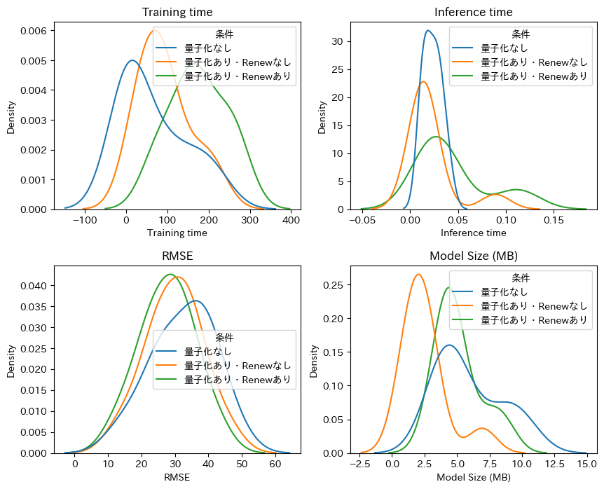
- Chen, T., & Guestrin, C. (2016). XGBoost: A Scalable Tree Boosting System. Proceedings of the 22nd ACM SIGKDD International Conference on Knowledge Discovery and Data Mining, 785–794. 10.1145/2939672.2939785