ベイズ線形回帰 - データサイエンス関連+αのメモ

import matplotlib.pyplot as plt
import numpy as np
import scipy as sp

# データを作成
n = 1000

from scipy.stats import multivariate_normal
mean = np.array([3, 5])
Sigma = np.array([
    [1, 0.5],
    [0.5, 2],
])
X = multivariate_normal.rvs(mean=mean, cov=Sigma, size=n, random_state=0)

import statsmodels.api as sm
X = sm.add_constant(X)

# 真のパラメータ
beta = np.array([2, 3, 4])

データが均一分散の場合¶

# 均一分散の場合
e = np.random.normal(loc=0, scale=1, size=n)
y = X @ beta + e

# 頻度主義
import statsmodels.api as sm
ols = sm.OLS(y, X).fit(cov_type="HC1")
ols.summary()

import pymc as pm
import arviz as az

model = pm.Model()
with model:
    beta0 = pm.Normal("beta0", mu=0, sigma=1)
    beta1 = pm.Normal("beta1", mu=0, sigma=1)
    beta2 = pm.Normal("beta2", mu=0, sigma=1)
    sigma = pm.HalfNormal("sigma", sigma=1)  # 分散なので非負の分布を使う

    # 平均値 mu
    mu = beta0 + beta1 * X[:, 1] + beta2 * X[:, 2]
    # 観測値をもつ確率変数は_obsとする
    y_obs = pm.Normal("y_obs", mu=mu, sigma=sigma, observed=y)

# モデルをGraphvizで表示
pm.model_to_graphviz(model)

WARNING (pytensor.tensor.blas): Using NumPy C-API based implementation for BLAS functions.

# ベイズ線形回帰モデルをサンプリング
with model:
    idata = pm.sample(
        chains=2,
        tune=1000, # バーンイン期間の、捨てるサンプル数
        draws=2000, # 採用するサンプル数
        random_seed=0,
    )

# 各chainsの結果を表示
az.plot_trace(idata, figsize=[4, 4])
plt.tight_layout()
plt.show()

Auto-assigning NUTS sampler...
Initializing NUTS using jitter+adapt_diag...
Multiprocess sampling (2 chains in 2 jobs)
NUTS: [beta0, beta1, beta2, sigma]

Sampling 2 chains for 1_000 tune and 2_000 draw iterations (2_000 + 4_000 draws total) took 10 seconds.
We recommend running at least 4 chains for robust computation of convergence diagnostics

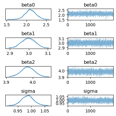
az.plot_posterior(idata)
plt.show()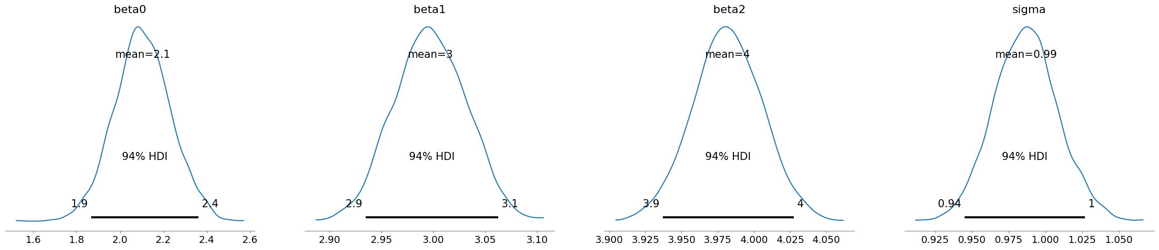

データが不均一分散の場合¶

# 不均一分散の場合
def normalize(x):
    return (x - x.min()) / (x.max() - x.min())

sigma = 1 + normalize(X[:, 1] + X[:, 2]) * 3
e = np.random.normal(loc=0, scale=sigma, size=n)
y = X @ beta + e

頻度主義 & 不均一分散に頑健な誤差推定¶

# 頻度主義
import statsmodels.api as sm
ols = sm.OLS(y, X).fit(cov_type="HC1")
ols.summary()

↑ 切片の推定にバイアスが入っている

均一分散を想定したベイズ線形回帰¶

import pymc as pm
import arviz as az

model = pm.Model()
with model:
    beta0 = pm.Normal("beta0", mu=0, sigma=1)
    beta1 = pm.Normal("beta1", mu=0, sigma=1)
    beta2 = pm.Normal("beta2", mu=0, sigma=1)
    sigma = pm.HalfNormal("sigma", sigma=1)  # 分散なので非負の分布を使う

    # 平均値 mu
    mu = beta0 + beta1 * X[:, 1] + beta2 * X[:, 2]
    # 観測値をもつ確率変数は_obsとする
    y_obs = pm.Normal("y_obs", mu=mu, sigma=sigma, observed=y)

# モデルをGraphvizで表示
pm.model_to_graphviz(model)

# ベイズ線形回帰モデルをサンプリング
with model:
    idata = pm.sample(
        chains=2,
        tune=1000, # バーンイン期間の、捨てるサンプル数
        draws=2000, # 採用するサンプル数
        random_seed=0,
    )

# 各chainsの結果を表示
az.plot_trace(idata, figsize=[4, 4])
plt.tight_layout()
plt.show()

Auto-assigning NUTS sampler...
Initializing NUTS using jitter+adapt_diag...
Multiprocess sampling (2 chains in 2 jobs)
NUTS: [beta0, beta1, beta2, sigma]

Sampling 2 chains for 1_000 tune and 2_000 draw iterations (2_000 + 4_000 draws total) took 10 seconds.
We recommend running at least 4 chains for robust computation of convergence diagnostics

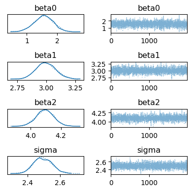
az.plot_posterior(idata)
plt.show()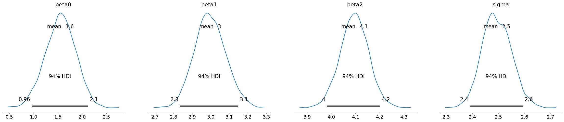

不均一分散を想定したベイズ線形回帰（WIP）¶

分散をxの関数にしたかった。以下コードで推定できるが個々の $\sigma_i$ が別々に推定される形になって結果が見づらい。もっといい表し方はないものか。

import pymc as pm
import arviz as az

model = pm.Model()
with model:
    beta0 = pm.Normal("beta0", mu=0, sigma=1)
    beta1 = pm.Normal("beta1", mu=0, sigma=1)
    beta2 = pm.Normal("beta2", mu=0, sigma=1)

    # 誤差分散にも線形モデルを入れる
    w0 = pm.Normal("w0", mu=0, sigma=1)
    w1 = pm.Normal("w1", mu=0, sigma=1)
    w2 = pm.Normal("w2", mu=0, sigma=1)
    lam = pm.math.exp(w0 + w1 * X[:, 1] + w2 * X[:, 2])
    sigma = pm.Exponential("sigma", lam=lam)  # 分散なので非負の分布を使う

    # 平均値 mu
    mu = beta0 + beta1 * X[:, 1] + beta2 * X[:, 2]
    # 観測値をもつ確率変数は_obsとする
    y_obs = pm.Normal("y_obs", mu=mu, sigma=sigma, observed=y)

# モデルをGraphvizで表示
pm.model_to_graphviz(model)

# ベイズ線形回帰モデルをサンプリング
with model:
    idata = pm.sample(
        chains=2,
        tune=1000, # バーンイン期間の、捨てるサンプル数
        draws=2000, # 採用するサンプル数
        random_seed=0,
    )

# 各chainsの結果を表示
az.plot_trace(idata, figsize=[4, 4])
plt.tight_layout()
plt.show()

az.plot_posterior(idata)
plt.show()

参考¶

Regression Models - Stan User’s Guide