輝度変換(intensity transformation) は画像の明るさに関する調整のこと。線形変換と非線形変換に大別される。
import cv2
import numpy as np
import matplotlib.pyplot as plt

img_path = 'sample_images/cat2.jpg'
img = cv2.imread(img_path)
img = cv2.cvtColor(img, cv2.COLOR_BGR2RGB)  # OpenCVはBGRなのでRGBに変換

plt.imshow(img)
plt.title("Original Image")
plt.show()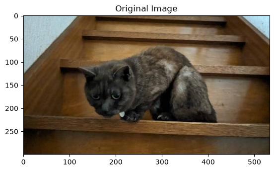
alpha = 1.5
beta = 50
bright_img = cv2.convertScaleAbs(img, alpha=alpha, beta=beta)
plt.imshow(bright_img)
plt.title(f"Linear Transformed (α={alpha}, β={beta})")
plt.show()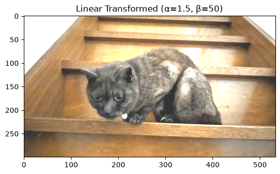
コントラストストレッチ(Contrast Stretching)
画像全体の明るさの範囲(ダイナミックレンジ)を最小値から最大値まで引き伸ばし、コントラストを強調する手法。
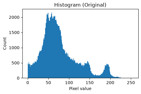
ヒストグラム(画素値の分布)が一部の範囲に偏っている(レンジが狭い)場合、その最小値・最大値を画素値の全域(例えば 0〜255)に均等に再マッピングすることで見やすくする。
img_gray = cv2.imread(img_path, cv2.IMREAD_GRAYSCALE)

fig, ax = plt.subplots(figsize=[5, 3])
ax.hist(img_gray.ravel(), bins=256, range=(0, 255))
ax.set_title("Histogram (Original)")
ax.set_xlabel("Pixel value")
ax.set_ylabel("Count")
fig.show()

print("min:", img_gray.min(), " max:", img_gray.max())
min: 0 max: 232
/tmp/ipykernel_622139/3215829073.py:8: UserWarning: FigureCanvasAgg is non-interactive, and thus cannot be shown
  fig.show()
# 最小値・最大値を画素値の全域(0-255)に再マッピングする
stretched_img = cv2.normalize(img_gray, None, alpha=0, beta=255, norm_type=cv2.NORM_MINMAX)

fig, axes = plt.subplots(ncols=2, nrows=2, figsize=[10, 6])
axes[0, 0].imshow(img_gray, cmap="gray")
axes[0, 0].set_title("Original Image")
axes[0, 1].imshow(stretched_img, cmap="gray")
axes[0, 1].set_title("Contrast Stretched Image")

axes[1, 0].hist(img_gray.ravel(), bins=256, range=(0, 255))
axes[1, 0].set_title("Histogram (Original)")
axes[1, 1].hist(stretched_img.ravel(), bins=256, range=(0, 255))
axes[1, 1].set_title("Histogram (Stretched)")
fig.tight_layout()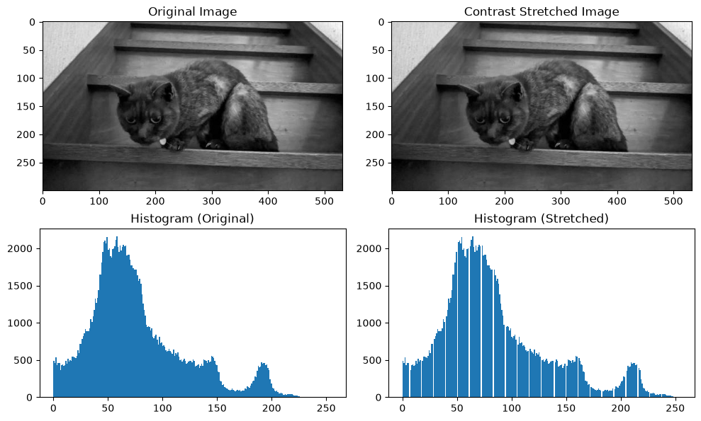
ヒストグラム平坦化
画像の濃度分布を均等にし、コントラストを最大化する。
img = cv2.imread(img_path, cv2.IMREAD_GRAYSCALE)
equ_img = cv2.equalizeHist(img)

fig, axes = plt.subplots(ncols=2, figsize=[10, 3])
axes[0].imshow(img, cmap="gray")
axes[0].set_title("Original Image")

axes[1].imshow(equ_img, cmap="gray")
axes[1].set_title("Equalized Image")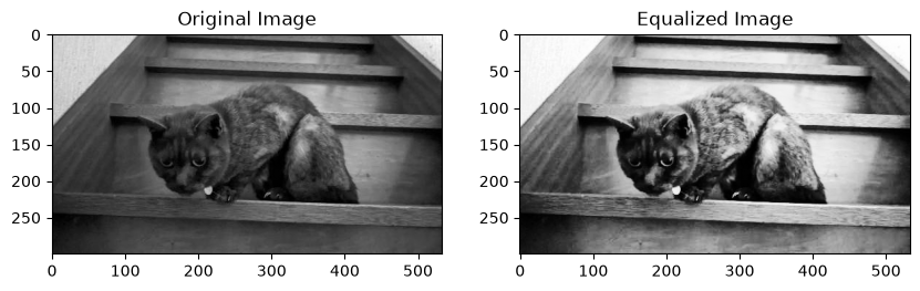
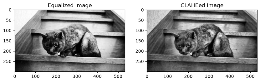
適用的ヒストグラム平坦化(CLAHE)
CLAHE(Contrast Limited Adaptive Histogram Equalization):局所的にコントラストを調整して細部も見やすくするequalizeHist
CLAHE は、局所的な領域ごとにヒストグラム均等化を行い、細部を見やすくする手法。
通常のヒストグラム均等化(cv2.equalizeHist())では、画像全体の明暗分布を一律に広げるが、CLAHEは小さなブロックごとに処理する。
処理の流れ
画像を小さな領域(タイル)に分割する
各タイルに対してヒストグラム均等化を行う
コントラストが高すぎる領域には「クリップ制限」をかける(= CLAHE の “CL”)
タイル間の境界を滑らかにするために補間(interpolation)を行う
参考
fig, axes = plt.subplots(ncols=2, figsize=[10, 3])
axes[0].imshow(equ_img, cmap="gray")
axes[0].set_title("Equalized Image")

# CLAHEオブジェクトを作成(clipLimit: コントラスト制限, tileGridSize: 分割数)
clahe = cv2.createCLAHE(clipLimit=2.0, tileGridSize=(8, 8))
# CLAHEを適用
cl_img = clahe.apply(img)

axes[1].imshow(cl_img, cmap="gray")
axes[1].set_title("CLAHEed Image")