フーリエ解析(Fourier analysis):信号を異なる周波数の正弦波(sin)の重ね合わせとして表現すること
例えば画像を周波数の表現にして、周波数をフーリエ解析で分解したりする。
幅Tの区間[−T/2,T/2]における連続関数f(t)はフーリエ級数に展開できる
f(t)=2a0+k=1∑∞(akcoskωot+bksinkωot),−2T≤t≤2T フーリエ係数は
ak=T2∫−T/2T/2f(t)coskωot dt,bk=T2∫−T/2T/2f(t)sinkωot dt である。
ここで
ωo=T2π である。これを 基本周波数 といい、フーリエ級数は関数f(t)をωoの整数倍の周波数の正弦波の重ね合わせとして表現する。
a0/2を 直流成分 と呼び、ωoのk倍の周波数の振動を第k 高調波 と呼ぶ。以下ではtを「時刻」とみなし、f(t)を「信号」と呼ぶ。
複素数の指数関数
複素数
複素数とは z=x+iy のように 実(数)部 x に 虚(数)部 y の i 倍を足したもの
i は 虚数単位 と呼ばれ、 i2=−1 となる数と約束したもの。
x軸を実部 x=Rez、y軸を 虚部 y=Imzにとった平面を 複素平面 と呼ぶ
import matplotlib.pyplot as plt
fig, ax = plt.subplots(figsize=(4, 3))

ax.arrow(-0.5, 0, 1.7, 0, head_width=0.05, head_length=0.1, fc='black', ec='black', length_includes_head=True)
ax.arrow(0, -0.5, 0, 1.5, head_width=0.05, head_length=0.1, fc='black', ec='black', length_includes_head=True)

ax.text(1.3, 0, "Re", fontsize=14, color='black')
ax.text(0, 1.1, "Im", fontsize=14, color='black')

ax.set_aspect('equal', adjustable='datalim')

ax.spines['top'].set_visible(False)
ax.spines['right'].set_visible(False)
ax.spines['left'].set_visible(False)
ax.spines['bottom'].set_visible(False)
ax.set(xticks=[], yticks=[])

c = 1 + 0.5j # 複素数
complex_points = [c, c.conjugate()] # conjugate: 共役複素数
colors = ['red', 'blue']

for i, (point, color) in enumerate(zip(complex_points, colors)):
    x, y = point.real, point.imag
    ax.plot([0, x], [0, y], color=color, linestyle='--', linewidth=0.8)
    ax.scatter([x], [y], color=color)
    z = r"$z$" if i == 0 else r"$\bar{z}$"
    ax.text(x + 0.05, y + 0.05, f'{z} = ${point}$', fontsize=10, color=color)


plt.show()
共役複素数
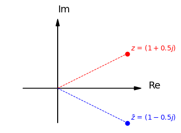
複素数 z=x+iy に対して, zˉ=x−iy をその 共役(きょうやく)複素数 といい、 z,zˉ は 互いに複素共役である という。
これらは複素平面上で x 軸に関して対称な位置にある。
この定義から
x=2z+zˉ,y=2iz−zˉ となる。また重要な関係として
zzˉ=(x+iy)(x−iy)=x2+y2=∣z∣2 が成り立つ。
オイラーの式
指数部が虚数の指数関数 eiθ を次の複素数と定義する。
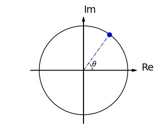
eiθ=cosθ+isinθ これは オイラーの式 と呼ばれる式で、複素平面の単位円上の実軸から角度θの点を表す。
定理
eiθeiϕ=ei(θ+ϕ) が成り立つ。
定義より次のように変形できる
eiθeiϕei(θ+ϕ)=(cosθ+isinθ)(cosϕ+isinϕ)=(cosθcosϕ−sinθsinϕ)+i(cosθsinϕ+sinθcosϕ)=cos(θ+ϕ)+isin(θ+ϕ) 両者が等しいことは、三角関数の加法定理
cos(θ+ϕ)sin(θ+ϕ)=cosθcosϕ−sinθsinϕ=cosθsinϕ+sinθcosϕ よりわかる
定理
cosθ=2eiθ+e−iθ,sinθ=2ieiθ−e−iθ が成り立つ。
オイラーの式 およびその式の θ を −θ に置き換えた式
eiθ=cosθ+isinθ,e−iθ=cosθ−isinθ を使うと、
eiθ+e−iθ=cosθ+isinθ+cosθ−isinθ=2cosθ より
cosθ=2eiθ+e−iθ が得られる。また
eiθ−e−iθ=cosθ+isinθ−cosθ+isinθ=2isinθ より
sinθ=2ieiθ−e−iθ が得られる。
フーリエ級数の複素表示
cosθ=2eiθ+e−iθ,sinθ=2ieiθ−e−iθ を使うと、フーリエ級数は以下のように表すことができる。
f(t)=2a0+k=1∑∞(ak2eikωot+e−ikωot+bk2ieikωot−e−ikωot)=2a0+21k=1∑∞((ak−ibk)eikωot+(ak+ibk)e−ikωot)=k=−∞∑∞Ckeikωot ただし
Ck=⎩⎨⎧(ak−ibk)/2a0/2(a−k+ib−k)/2k>0k=0k<0 である
また、Ckの各式は次のように変形できる
2ak−ibk2a02a−k+ib−k=T2∫−T/2T/2f(t)2coskωot−isinkωot dt=T1∫−T/2T/2f(t)e−ikωot dt=T1∫−T/2T/2f(t)dt=T2∫−T/2T/2f(t)2cos(−kωot)+isin(−kωot) dt=T1∫−T/2T/2f(t)(coskωot−isinkωot)dt=T1∫−T/2T/2f(t)e−ikωot dt f(t)=k=−∞∑∞Ckeikωot,Ck=T1∫−T/2T/2f(t)e−ikωot dt このCkを (複素)フーリエ係数 と呼ぶ。
info - Unknown Directive
$f(t)$は実数なのに、フーリエ係数は複素数なのは問題ないのか?

→ $C_k$と$e^{i k \omega_o t}$は共役複素数なので掛けると虚部が消えて実数になる
info - Unknown Directive
位相(波の数)は角度として表される。

特に複素平面上で単位円を考えると、位相は単位円の角度(回転)として表される
import numpy as np
import matplotlib.pyplot as plt
fig, ax = plt.subplots(figsize=(4, 3))

# 軸を描画
ax.arrow(-1.2, 0, 2.4, 0, head_width=0.05, head_length=0.1, fc='black', ec='black', length_includes_head=True)
ax.arrow(0, -1.2, 0, 2.4, head_width=0.05, head_length=0.1, fc='black', ec='black', length_includes_head=True)

ax.text(1.3, 0, "Re", fontsize=14, color='black')
ax.text(0, 1.3, "Im", fontsize=14, color='black')

ax.set_aspect('equal', adjustable='datalim')
ax.spines['top'].set_visible(False)
ax.spines['right'].set_visible(False)
ax.spines['left'].set_visible(False)
ax.spines['bottom'].set_visible(False)
ax.set(xticks=[], yticks=[])


# 単位円
theta = np.linspace(0, 2*np.pi, 100)
x = np.cos(theta)
y = np.sin(theta)
plt.plot(x, y, 'k-', linewidth=1)  # 黒い実線で単位円を描画

# curve
t = 0.3*np.pi
theta = np.linspace(0, t, 100)
x = np.cos(theta) * 0.2
y = np.sin(theta) * 0.2
ax.plot(x, y, 'k--', linewidth=1)  # 黒い実線で単位円を描画

# text
m = len(x) // 2
ax.text(x[m], y[m], r"$\theta$")

# line
x = np.cos(t)
y = np.sin(t)
ax.plot([0, x], [0, y], color="blue", linestyle='-.', linewidth=0.8)
ax.scatter([x], [y], color="blue")

plt.show()
フーリエ変換
フーリエ級数
f(t)=k=−∞∑∞Ckeikωot,Ck=T1∫−T/2T/2f(t)e−ikωot dt において
ωk=kωo,k=0,±1,±2,… とおき、
Δω=ωk+1−ωk=ωo=T2π,Ck=TF(ωk) と書くと、
f(t)=2π1k=−∞∑∞F(ωk)eiωktΔω,F(ωk)=∫−T/2T/2f(t)e−iωkt dt となる。周期T→∞とすると、Δω→0となり、積分として表すことができる。
F(ω)=∫−∞∞f(t)e−iωt dt を信号f(t)の フーリエ変換 と呼び、
f(t)=2π1∫−∞∞F(ω)eiωt dω を 逆フーリエ変換 と呼ぶ。
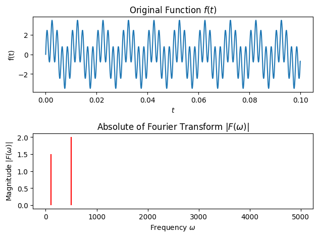
図:フーリエ変換のイメージ。F(ω)は一般に複素数なのでグラフに書けない → 絶対値をとる
import numpy as np
import matplotlib.pyplot as plt

# サンプルデータを生成する
N = 1000
d = 0.0001 # サンプリング周期
t = np.arange(0, N * d, d) # 時間

def f(t):
    freq1, freq2 = 100, 500  # 周波数
    s1, s2 = 1.5, 2 # スペクトル F(ω)
    return s1 * np.sin(2 * np.pi * t * freq1) + s2 * np.sin(2 * np.pi * t * freq2)

y = f(t)
F = np.fft.fft(y) # フーリエ変換
freq = np.fft.fftfreq(N, d=d)  # 周波数スケール

# 振幅スペクトル Amplitude の取得
# 振幅スペクトルは信号をフーリエ変換した結果の絶対値をとったもの
Amp = np.abs(F)
Amp = Amp / (N / 2) # 正規化

# 結果をプロット
fig, axes = plt.subplots(nrows=2)
axes[0].plot(t, y)
axes[0].set(title=r'Original Function $f(t)$', xlabel=r"$t$", ylabel=r"f(t)")

# 左右対称なので正の値だけ N//2 で取り出す
axes[1].stem(freq[:N//2], Amp[:N//2], 'r', markerfmt=" ", basefmt=" ")
axes[1].set(title=f'Absolute of Fourier Transform $|F(\omega)|$', xlabel=r'Frequency $ω$', ylabel=r'Magnitude $|F(ω)|$')

fig.tight_layout()
fig.show()
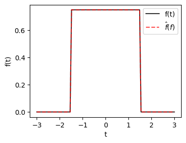
次の関数は幅Wの 矩形窓(rectangular window) と呼ばれる
w(t)={1/2W0−W≤t≤W それ以外 このフーリエ変換は
W(ω)=2W1∫−WWe−iωt dt=2W1∫−WW(cosωt−isinωt)dt(オイラーの式よりe−iωt=cosωt−isinωt)=2W1(∫−WWcosωt dt−∫−WWisinωt dt)(∵積分の線形性)=2W1∫−WWcosωt dt(∵sinは奇関数すなわちsin(−θ)=−sin(θ)であり、−Wから+Wまで積分したら0になるため消える)=W1∫0Wcosωt dt(∵∫−WWcosωt dt=2∫0Wcosωt dt)=W1[ωsinωt]0W(∵∫cos(ωt)dt=ωsin(ωt))=W1(ωsinωW−ωsin0)=WωsinWω(∵sin0=0)=sincπWω となる。ただし、
sincx:=πxsinπx と定義する。
# 参考:numpyの高速フーリエ変換 fft を使う場合
# 自分で離散的なデータポイントからフーリエ変換するのは離散フーリエ変換を学んでからやる
import numpy as np
import matplotlib.pyplot as plt

fig, ax = plt.subplots(figsize=(4, 3))

# もとの関数 f(t)
w = 1.5  # width
def f(t):
    return (1/2*w) * 1 * ((-w <= t) & (t <= w))

t = np.linspace(-3, 3, 100)
y = f(t)
ax.plot(t, f(t), label="f(t)", color="black", alpha=0.8)

# フーリエ変換 F(omega)
fourier = np.fft.fft(y)
inv_fourier = np.fft.ifft(fourier).real  # 実部のみ
ax.plot(t, inv_fourier, label=r"$\hat{f}(f)$", color="red", linestyle="--", alpha=0.7)

ax.set(xlabel="t", ylabel="f(t)")
ax.legend()
plt.show()
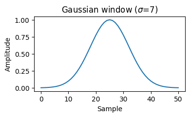
次の関数w(t) を幅σの ガウス窓(Gaussian window) という。
w(t)=2πσ1e−t2/2σ2 このフーリエ変換は
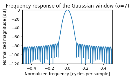
W(ω)=∫−∞∞w(t)e−iωt dt=2πσ1∫−∞∞e−t2/2σ2e−iωt dt=2πσ1∫−∞∞e−(2σ2t2+iωt) dt(指数法則anam=an+m)=2πσ1∫−∞∞e−(t+iσ2ω)2/2σ2−σ2ω2/2 dt(平方完成したり色々いじるとこうなる)=(2πσ1∫−∞∞e−(t+iσ2ω)2/2σ2 dt)e−σ2ω2/2 ここで z=t+iσ2ωと変数変換すると
W(ω)=(2πσ1∫−∞∞e−z2/2σ2 dz)e−σ2ω2/2=e−σ2ω2/2=σ2π(2πσ−11e−ω2/2σ−2) となる
from scipy import signal
import matplotlib.pyplot as plt
window = signal.windows.gaussian(51, std=7)
fig, ax = plt.subplots(figsize=(4, 2))
ax.plot(window)
ax.set(title=r"Gaussian window ($\sigma$=7)", ylabel="Amplitude", xlabel="Sample")
fig.show()
import numpy as np
from scipy import signal
from scipy.fft import fft, fftshift
import matplotlib.pyplot as plt

fig, ax = plt.subplots(figsize=(4, 2.4))

window = signal.windows.gaussian(51, std=7)
A = fft(window, 2048) / (len(window)/2.0)
freq = np.linspace(-0.5, 0.5, len(A))
response = 20 * np.log10(np.abs(fftshift(A / abs(A).max())))
ax.plot(freq, response)
ax.plot(window)
ax.set(title=r"Frequency response of the Gaussian window ($\sigma$=7)",
       ylabel="Normalized magnitude [dB]", xlabel="Normalized frequency [cycles per sample]",
       xlim=(-0.5, 0.5), ylim=(-120, 0))
fig.show()
畳み込み積分
(左辺の積分におけるfとgの変数の和がs+t−s=tとなっている)
畳み込み積分は分配法則、交換法則、結合法則が成り立つ
分配法則: f(t)∗(ag(t)+bh(t))=af(t)∗g(t)+bf(t)∗h(t)
交換法則:f(t)∗g(t)=g(t)∗f(t)
結合法則:(f(t)∗g(t))∗h(t)=f(t)∗(g(t)∗h(t))
f(t)∗g(t)のフーリエ変換は次のようになる
∫−∞∞f(t)∗g(t)e−iωt dt=∫−∞∞(∫−∞∞f(s)g(t−s)ds)e−iωt dt=∫−∞∞f(s)(∫−∞∞g(t−s)e−iωt dt)ds=∫−∞∞f(s)(∫−∞∞g(t′)e−iω(t′+s)dt′)ds=∫−∞∞f(s)(∫−∞∞g(t′)e−iωt′dt′)e−iωs ds=(∫−∞∞f(s)e−iωs ds)(∫−∞∞g(t′)e−iωt′dt′)=F(ω)G(ω) (積分の順序を入れ換え、 t′=t−s と変数変換し、 t=t′+s を代入した)
一般に、ある集合に要素間の演算が定義されているものを 代数系 と呼ぶ。そして2つの異なる集合での演算が同じ規則に従うとき、2つの代数系は 同型 であるという。
関数の和+と畳み込み積分∗に関する演算は、そのフーリエ変換の和+と積×に関する演算と同じであり、両方の代数系が同型である。
フィルター
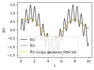
信号 f(t) の値を時刻 t をはさむ幅 2W の区間で平均し、これを f~(t) と定義する。
f~(t):=2W1∫−WWf(t−s)ds 矩形窓やガウス窓w(t)を使うと、次のように書き直すことができる
f~(t)=∫−∞∞w(s)f(t−s)ds=w(t)∗f(t) これにより、関数w(t)を様々な関数に変えれば信号f(t)の様々な変換ができる。このような操作を関数w(t)による フィルター という。
w(t),f(t)のフーリエ変換をそれぞれW(ω),F(ω)とおけば、畳み込み積分の定理によりf~(t)=w(t)∗f(t)のフーリエ変換は
F~(ω)=W(ω)F(ω) と書くことができる。
もし∣ω∣が小さい部分で∣W(ω)∣が大きく、∣ω∣が大きい部分で∣W(ω)∣が小さくなる場合、w(t)によるフィルターは低周波成分を増幅し、高周波成分を減衰させる。このようなフィルターを ローパスフィルター ( 低域フィルター )と呼ぶ。その逆のフィルターを ハイパスフィルター ( 高域フィルター )と呼ぶ。
その中間として、特定の∣ω∣の付近を増幅し、それ以外を減衰させるフィルターは 帯域フィルター ( バンドパスフィルター )と呼ぶ。
import numpy as np
import matplotlib.pyplot as plt

N = 1000
t = np.linspace(0, 10, N)

def f(t):
    return np.sin(t) + 0.5 * np.sin(10 * t)

signal = f(t)

fig, ax = plt.subplots(figsize=(4, 3))
ax.plot(t, signal, label="f(t)", color="black", alpha=0.8)
ax.set(xlabel="t", ylabel="f(t)")

from scipy.signal.windows import gaussian
from scipy.signal import fftconvolve

def gaussian_smoothing(signal, window_size, std_dev):
    # ガウス窓を作成
    gauss_window = gaussian(window_size, std=std_dev)
    gauss_window /= gauss_window.sum()  # 窓の正規化
    # 畳み込み
    return fftconvolve(signal, gauss_window, mode='same')  # 同じ長さを保つ

smoothed_signal = gaussian_smoothing(signal, window_size=N//2, std_dev=100)
ax.plot(t, smoothed_signal, label=r"$\tilde{f}(t)$", color="steelblue", alpha=0.8)

# scipy
from scipy.ndimage import gaussian_filter1d
smoothed_signal = gaussian_filter1d(signal, 100)
ax.plot(t, smoothed_signal, label=r"$\tilde{f}(t)$ (scipy gaussian_filter1d)", color="orange", alpha=0.8)

ax.legend()
fig.show()
∫−∞∞f(t)g(t) dt=2π1∫−∞∞F(ω)G(ω) dω については、
∫−∞∞f(t)g(t)dt=∫−∞∞f(t)(2π1∫−∞∞G(ω)e−iωt dω)dt=2π1∫−∞∞(∫−∞∞f(t)e−iωt dt)G(ω)dω=2π1∫−∞∞F(ω)G(ω)dω g(t)=f(t)とすると
∫−∞∞∣f(t)∣2 dt=2π1∫−∞∞∣F(ω)∣2 dω が得られる
信号f(t)が時間tとともに変動する振動を表すとき、∣f(t)∣2はその振動の単位時間あたりの エネルギー とみなすことができる。
パーセバルの第2式
∫−∞∞∣f(t)∣2 dt=2π1∫−∞∞∣F(ω)∣2 dω はエネルギーがすべてのωにわたる∣F(ω)∣2の積分で表されることを意味する。
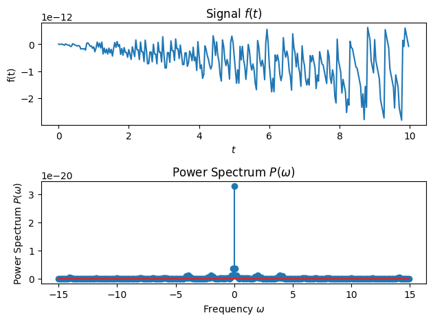
これを パワースペクトル と呼び、
P(ω)=∣F(ω)∣2 は周波数ωの振動成分のもつエネルギーであると解釈できる。
フーリエ変換F(ω)は一般に複素数だが、その絶対値は実数になりグラフに描くことができる。
フーリエ変換は共役F(−ω)=F(ω)であり∣F(−ω)∣=∣F(ω)∣だから、パワースペクトルはグラフにすると原点を中心に左右対称になる。
# うまくいかなかった
import numpy as np
import matplotlib.pyplot as plt

sampling_rate = 30
duration = 10
N = int(sampling_rate * duration)

t = np.linspace(0, duration, N, endpoint=False)
frequencies = [30, 60, 90, 150, 300]
amplitudes = [1.0, 0.8, 0.6, 0.4, 0.2]
signal = sum(
    amp * np.sin(2 * np.pi * freq * t) for freq, amp in zip(frequencies, amplitudes)
)

# Perform the Fourier Transform
fft_result = np.fft.fft(signal)
frequencies = np.fft.fftfreq(len(signal), 1 / sampling_rate)
power_spectrum = np.abs(fft_result)**2

# 結果をプロット
fig, axes = plt.subplots(nrows=2)
axes[0].plot(t, signal)
axes[0].set(title=r'Signal $f(t)$', xlabel=r"$t$", ylabel=r"f(t)")
axes[1].stem(frequencies[:len(frequencies)], power_spectrum[:len(frequencies)])
# axes[1].stem(frequencies[:len(frequencies)//2], power_spectrum[:len(frequencies)//2])
axes[1].set(title=f'Power Spectrum $P(\omega)$', xlabel=r'Frequency $ω$', ylabel=r'Power Spectrum $P(ω)$')
fig.tight_layout()
fig.show()
複素計量空間(ユニタリ空間)とのつながり
信号f,gの内積を
(f,g):=∫−∞∞f(t)g(t) dt と定義すれば、ノルムも
∥f∥=(f,f) と定義でき、フーリエ変換も
(F,G):=2π1∫−∞∞F(ω)G(ω)dω とおけば
∥F∥=2π1∫−∞∞∣F(ω)∣2 dω となり、パーセバルの式は
(f,g)=(F,G),∥f∥2=∥F∥2 とシンプルでエレガントな表記にすることができる。
この内積は計量ベクトル空間の内積の公理のうち対称性(f,g)=(g,f)を満たさないが、ユニタリ空間におけるエルミート対称性(f,g)=(g,f)は満たす。つまり、ユニタリ空間上で考えるなら上のシンプルな表記が可能。
自己相関関数
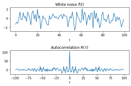
R(0) は信号 f(t) のエネルギー ∫−∞∞∣f(t)∣2 dt に等しく、通常は大きな値をとる。
∣τ∣ が大きくなると R(τ) は急速に減衰する。
import numpy as np
from scipy import signal
rng = np.random.default_rng()
sig = rng.standard_normal(100)
autocorr = signal.fftconvolve(sig, sig[::-1], mode='full')

import matplotlib.pyplot as plt
fig, (ax_orig, ax_mag) = plt.subplots(2, 1, dpi=72, figsize=[6, 4])
ax_orig.plot(sig)
ax_orig.set(title=f'White noise $f(t)$', xlabel=r"$t$")
ax_mag.plot(np.arange(-len(sig)+1,len(sig)), autocorr)
ax_mag.set(title=r'Autocorrelation $R(\tau)$', xlabel=r"$\tau$")
fig.tight_layout()
fig.show()
なぜ自己相関関数と呼ぶのか
実数の信号 f(t),g(t) の内積 ∫−∞∞f(t)g(t)dt の場合、f(t)とg(t)が無関係ならf(t)g(t)はそれぞれプラスとマイナスで打ち消し合ったりして小さい値になるが、f(t)とg(t)が似てるならf(t)g(t)≈f(t)2≥0となり、積分すると大きな値になる。
複素数の信号の場合はエルミート内積∫−∞∞f(t)g(t)dtを考えると、もしf(t)とg(t)が似てるならf(t)g(t)≈f(t)f(t)≈∣f(t)∣2≥0となり、積分すると大きな値になる。
このように、内積・エルミート内積は類似度の尺度となり、 (相互)相関 と呼ばれる。
f(t) と、それをτだけ平行移動した f(t−τ) の類似度なので自己相関と呼ばれる。
自己相関関数の性質
R(−τ)=R(τ),∣R(−τ)∣=∣R(τ)∣
第1式は
R(−τ)=∫−∞∞f(t)f(t+τ)dt=∫−∞∞f(t′−τ)f(t′)dt′=∫−∞∞f(t′)f(t′−τ)dt′=R(τ) で示される。また共役複素数をとっても絶対値は変化しないため第2式が成り立つ。
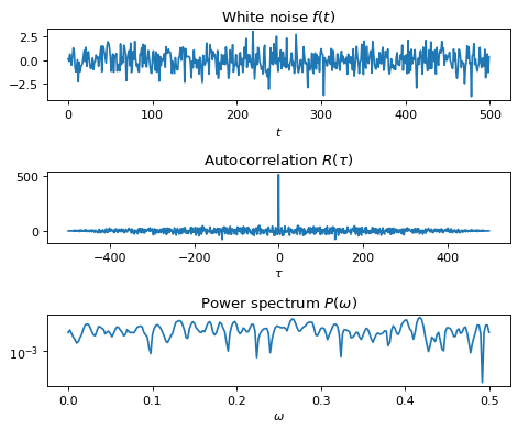
よってパワースペクトルを算出するには、2通りの方法がある
信号f(t)のフーリエ変換F(ω)を計算して絶対値の2乗を取る
自己相関関数R(τ)を計算してフーリエ変換する
信号を精度よく積分するのは難しいため、自己相関関数で算出するほうが実用上は便利らしい
import numpy as np
from scipy import signal
rng = np.random.default_rng(seed=0)
sig = rng.standard_normal(500)

autocorr = signal.fftconvolve(sig, sig[::-1], mode='full')

import matplotlib.pyplot as plt
fig, axes = plt.subplots(3, 1, dpi=80, figsize=[6, 5])
axes[0].plot(sig)
axes[0].set(title=f'White noise $f(t)$', xlabel=r"$t$")

n = len(sig)
x = np.arange(-n+1, n)
axes[1].plot(x, autocorr)
axes[1].set(title=r'Autocorrelation $R(\tau)$', xlabel=r"$\tau$")

# Power spectrum
omega, P = signal.periodogram(sig, window='flattop', scaling='spectrum')
axes[2].semilogy(omega, P)
axes[2].set(title=r'Power spectrum $P(\omega)$', xlabel=r"$\omega$")

fig.tight_layout()
fig.show()
from scipy import signal, fft
import matplotlib.pyplot as plt
fig, axes = plt.subplots(2, 1, dpi=80, figsize=[6, 4])
axes[0].plot(sig)
axes[0].set(title=f'White noise $f(t)$', xlabel=r"$t$")

n = len(sig)
T = 1
F = fft.fft(sig, len(sig))[:n//2]
omega = fft.fftfreq(n, T)[:n//2]
P = np.abs(F) ** 2

# Power spectrum from F(ω)
axes[1].semilogy(omega, P)
axes[1].set(title=r'Power spectrum $P(\omega)$ from $F(\omega)$', xlabel=r"$\omega$")

fig.tight_layout()
fig.show()
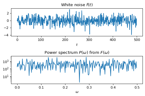
それっぽいやつやってみたがうまくPが一致しない
そもそもホワイトノイズのPは1のはず…
サンプリング定理
信号 f(t) の離散的な点 {tk},k=0,±1,±2,±3,… での値 {fk} を サンプル点 {tk} での サンプル値 と呼ぶ。
サンプル点 {tk} の間隔 τ を サンプル間隔 と呼ぶ。サンプル値 {fk} のみから連続関数を再現することを 補間 という。
次の性質を持つ関数 ϕ(t) をサンプル間隔 τ の 補間関数 と呼ぶ
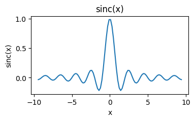
ϕ(t)={10t=0t=±τ,±2τ,±3τ,… 補間関数の例はsinc(cardinal sine)関数
sinc(x)=πxsinπx
import numpy as np
import matplotlib.pyplot as plt

def sinc(x):
    return np.sin(np.pi * x) / (np.pi * x)

fig, ax = plt.subplots(figsize=[4,2])

x = np.linspace(-3*np.pi, 3*np.pi, 100)
ax.plot(x, sinc(x))
ax.set(title="sinc(x)", xlabel="x", ylabel="sinc(x)")
fig.show()
f^(t)=k=−∞∑∞fkϕ(t−tk) はすべてのサンプル点tiでサンプルの値fiをとる
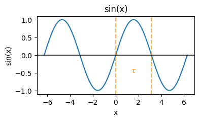
サンプリング間隔τを半周期(波1つ分。sinならπの幅)とする振動は各周波数W=π/τを持つ
import numpy as np
import matplotlib.pyplot as plt

fig, ax = plt.subplots(figsize=[4,2])
x = np.linspace(-2*np.pi, 2*np.pi, 100)
ax.plot(x, np.sin(x))
ax.set(title="sin(x)", xlabel="x", ylabel="sin(x)")
ax.axhline(0, color="black", alpha=0.7)

ax.axvline(0, color="darkorange", linestyle="--", alpha=0.7)
ax.axvline(np.pi, color="darkorange", linestyle="--", alpha=0.7)
ax.text(np.pi / 2, -0.5, r"$\tau$", color="darkorange", ha="center")

fig.show()
信号f(t)のフーリエ変換は
f(t)=2π1∫−∞∞F(ω)eiωt dω,F(ω)=∫−∞∞f(t)e−iωt dt となる。F(ω)は区間[−W,W]でフーリエ級数に展開できる
F(ω)=k=−∞∑∞Ckeiπkω/W,Ck=2W1∫−WWF(ω)e−iπkω/W dω 区間 [−W,W] の外では F(ω)=0 であるから、 Ck は次のように計算できる。
Ck=2W1∫−∞∞F(ω)e−iπkω/W dω=Wπ2π1∫−∞∞F(ω)eiω(−πk/W)dω=Wπf(−Wπk)=τf(−kτ)=τf−k よってF(ω)は区間[−W,W]で
F(ω)=k=−∞∑∞τf−keiπkω/W=τk=−∞∑∞fke−iπkω/W=τk=−∞∑∞fke−ikτω=τk=−∞∑∞fke−itkω となる。
まとめると、
f(t)=2π1∫−WWF(ω)eiωt dω=2π1∫−WW(τk=−∞∑∞fke−itkω)eiωt dω=2πτk=−∞∑∞fk∫−WWei(t−tk)ωdω=2πτk=−∞∑∞fk∫−WW(cos(t−tk)ω+isin(t−tk)ω)dω=πτk=−∞∑∞fk∫0Wcos(t−tk)ωdω=W1k=−∞∑∞fk∫0Wcos(t−tk)ωdω(∵τ=π/W)=W1k=−∞∑∞fk[(t−tk)sin(t−tk)ω]0W=k=−∞∑∞fkW(t−tk)sinW(t−tk)=k=−∞∑∞fksincπW(t−tk)=k=−∞∑∞fksincτt−tk 一定の条件を満たす間隔で得られたサンプルと、一定の条件を満たす信号は、 離散的なサンプルからもとの連続的な信号を再現できる というのがサンプリング定理。
音声などの信号に限らず、デジタル画像などアナログ(連続値)なものをデジタル(離散値)にサンプリングする分野で広く応用されている。
間隔τでサンプリングするとW=π/τ以上の周波数の信号は捉えられない。W=π/τをサンプリング間隔τに対する ナイキスト周波数 とよぶ。
import numpy as np
import matplotlib.pyplot as plt

def approx(x, tau):
    # tau: サンプリング周期
    # 間隔を指定してのサンプリングが難しかったのでarangeで生成
    x_samples = np.arange(-3 * np.pi, 3 * np.pi, tau)
    y_samples = np.sin(x_samples)

    y_hat = []
    for i in range(len(x)):
        y_hat_i = 0
        for j in range(len(y_samples)):
            y_hat_i += y_samples[j] * np.sinc((x[i] - x_samples[j]) / tau)
        y_hat.append(y_hat_i)
    return x_samples, y_samples, np.array(y_hat)

taus = [
    ("\pi", np.pi),
    ("\pi/1.1", np.pi/1.1),
    ("\pi/2", np.pi/2),
]
fig, axes = plt.subplots(figsize=[12, 2.5], ncols=len(taus), sharey=True)
for i, ax in enumerate(axes):
    # true signal
    x = np.arange(-3 * np.pi, 3 * np.pi, 0.1)
    y = np.sin(x)
    ax.plot(x, y, label=r"true signal $f(t)$", color="black", alpha=0.7)

    # approximate
    tau_str, tau = taus[i]
    x_samples, y_samples, y_hat = approx(x, tau=tau)
    ax.plot(x_samples, y_samples, label=r"samples", alpha=0.8, linestyle=":", marker=".")
    ax.plot(x, y_hat, label=rf"approximation ($\tau = {tau_str}$)", alpha=0.8, linestyle="--")
    ax.set(xlabel=r"$t$", title=rf"Approximation ($\tau = {tau_str} = {tau:.2f}$)")#, ylim=(-1.2, 3.2))
    ax.legend()
    if i == 0:
        ax.set(ylabel=r"$f(t)$")

fig.show()
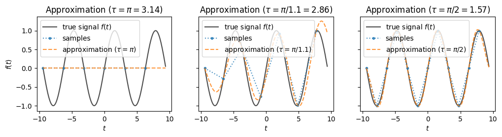
周期TがT=2τなら、周波数がω=2π/T=π/τ=W
1周期がT=2τ=2πのsinに対してサンプリング間隔がτ=πだとナイキスト周波数であり、もとの信号が復元できない様子。ω=2π/T=2π/2π=1…?