メトロポリス・ヘイスティング（MH）法

"""
Metropolis-Hastings
- モデル: y_i ~ Normal(mu, sigma^2), 既知sigma
- 事前:   mu ~ Normal(0, tau^2)
→ 事後 p(mu|y) を MCMC でサンプリング

ポイント:
- 正規化定数は不要（log事後の差だけ使う）
- 受理率(acceptance rate)と提案分布幅(step)で挙動が変わる
"""

import numpy as np
import matplotlib.pyplot as plt


# -----------------------------
# 1) データ生成（学習用に真値から作る）
# -----------------------------
rng = np.random.default_rng(0)
mu_true = 1.5
sigma = 1.0
n = 50
y = rng.normal(loc=mu_true, scale=sigma, size=n)

# 事前（mu ~ N(0, tau^2)）
tau = 3.0


# -----------------------------
# 2) log事後（正規化定数は捨ててOK）
#    log p(mu|y) = log p(y|mu) + log p(mu) + const
# -----------------------------
def log_posterior(mu: float, y: np.ndarray, sigma: float, tau: float) -> float:
    # log likelihood: sum_i log N(y_i | mu, sigma^2)
    # 定数項 -0.5*log(2πσ^2) は差分で消えるので省略して良い
    ll = -0.5 * np.sum(((y - mu) / sigma) ** 2)

    # log prior: log N(mu | 0, tau^2) も定数は省略して良い
    lp = -0.5 * ((mu / tau) ** 2)

    return ll + lp


# -----------------------------
# 3) Metropolis-Hastings（ランダムウォーク提案）
#    mu' = mu + Normal(0, step^2)
# -----------------------------
def metropolis_hastings(
    y: np.ndarray,
    sigma: float,
    tau: float,
    n_samples: int = 20_000,
    burn_in: int = 2_000,
    step: float = 0.5,
    init: float = 0.0,
    seed: int = 123,
):
    rng = np.random.default_rng(seed)

    samples = np.empty(n_samples, dtype=float)

    mu = float(init)
    logp = log_posterior(mu, y, sigma, tau)

    accepted = 0

    for t in range(n_samples):
        # 提案
        mu_prop = mu + rng.normal(0.0, step)
        logp_prop = log_posterior(mu_prop, y, sigma, tau)

        # 受理確率: alpha = min(1, exp(logp_prop - logp))
        # 数値安定のため、log空間で比較する
        log_alpha = logp_prop - logp

        if np.log(rng.random()) < log_alpha:
            mu = mu_prop
            logp = logp_prop
            accepted += 1

        samples[t] = mu

    acc_rate = accepted / n_samples

    # burn-in を捨てて返す
    post = samples[burn_in:]
    return post, samples, acc_rate


# -----------------------------
# 4) 実行
# -----------------------------
post, trace, acc_rate = metropolis_hastings(
    y=y,
    sigma=sigma,
    tau=tau,
    n_samples=30_000,
    burn_in=3_000,
    step=0.6,   # ←ここを変えると挙動が変わる（重要）
    init=0.0,
    seed=42,
)

print(f"acceptance rate = {acc_rate:.3f}")
print(f"posterior mean  = {post.mean():.3f}")
print(f"posterior sd    = {post.std(ddof=1):.3f}")


# -----------------------------
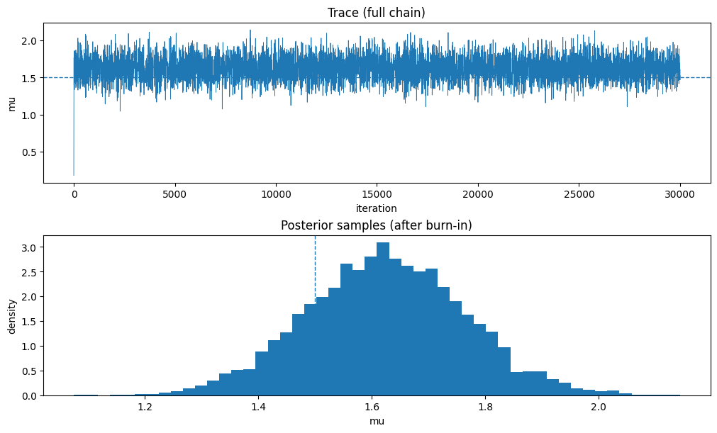
# 5) 可視化（トレース & ヒストグラム）
# -----------------------------
fig, ax = plt.subplots(2, 1, figsize=(10, 6), constrained_layout=True)

ax[0].plot(trace, linewidth=0.6)
ax[0].axhline(mu_true, linestyle="--", linewidth=1.0)
ax[0].set_title("Trace (full chain)")
ax[0].set_xlabel("iteration")
ax[0].set_ylabel("mu")

ax[1].hist(post, bins=50, density=True)
ax[1].axvline(mu_true, linestyle="--", linewidth=1.0)
ax[1].set_title("Posterior samples (after burn-in)")
ax[1].set_xlabel("mu")
ax[1].set_ylabel("density")

plt.show()