回帰 Regression
絶対損失
二乗しないため外れ値に強い(外れ値の予測誤差を比較的小さく評価する)。
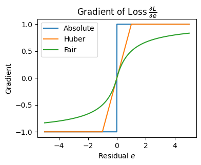
勾配
では微分が定義されないため、劣勾配(subgradient) として区間 を取る
実装上は多くの場合、 とし、 の場合は 0 を返すことが多い
Source
import matplotlib.pyplot as plt
import numpy as np

e = np.linspace(-4, 4, 100)

plt.figure(figsize=[4, 3])
plt.plot(e, (1/2) * e**2, label=r"Squared Loss $\frac{1}{2}e^2$")
plt.plot(e, abs(e), label=r"Absolute Loss $|e|$")

plt.ylabel("Loss")
plt.xlabel(r"Residual $e$")
plt.legend()
plt.show()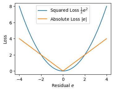
Fair loss
Fair loss は、残差が大きくなるにつれて影響を連続的になだらかに抑制するロバスト損失関数である。
Huber loss のような明確な折れ点を持たず、全域で滑らかな形状を持つ。
勾配
特徴
小さな残差では二乗誤差に近い挙動
残差が大きくなるにつれて勾配が連続的に減衰
全域で滑らか(高階微分も連続)
非常に大きな外れ値に対しても安定
利用場面
外れ値が多い、または裾の重い分布を持つデータ
勾配ベース最適化で数値安定性を重視する場合
Huber loss よりも強いロバスト性が必要なケース
Source
import matplotlib.pyplot as plt
import numpy as np

e = np.linspace(-5, 5, 1000)
# parameters
delta = 1.0
c = 1.0
# Huber loss
huber = np.where(
    np.abs(e) <= delta,
    0.5 * e**2,
    delta * (np.abs(e) - 0.5 * delta)
)
# Fair loss
fair = c**2 * (np.abs(e) / c - np.log(1 + np.abs(e) / c))

plt.figure(figsize=[4,3])

plt.plot(e, abs(e), label=r"Absolute loss")
plt.plot(e, huber, label="Huber loss")
plt.plot(e, fair, label="Fair loss")
plt.xlabel("Residual $e$")
plt.ylabel("Loss")
plt.legend()
plt.show()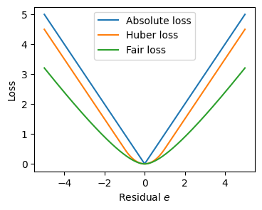
Source
import matplotlib.pyplot as plt
import numpy as np

e = np.linspace(-5, 5, 1000)

# parameters
delta = 1.0
c = 1.0

# gradients

# Absolute loss gradient (subgradient, 0 at e=0)
grad_abs = np.sign(e)

# Huber loss gradient
grad_huber = np.where(
    np.abs(e) <= delta,
    e,
    delta * np.sign(e)
)

# Fair loss gradient
grad_fair = e / (1 + np.abs(e) / c)

# plot
plt.figure(figsize=(4, 3))
plt.title(r"Gradient of Loss $\frac{\partial L}{\partial e}$")
plt.plot(e, grad_abs, label=r"Absolute")
plt.plot(e, grad_huber, label="Huber")
plt.plot(e, grad_fair, label="Fair")
plt.xlabel("Residual $e$")
plt.ylabel("Gradient")
plt.legend()
plt.show()