LASSO - データサイエンス関連+αのメモ

$n$ 個のサンプルと $m$ 個の特徴量からなる特徴量の行列 $\boldsymbol{X}$ を用いて目的変数 $\boldsymbol{y}$ を近似する線形モデル

\newcommand{\b}[1]{\boldsymbol{#1}} \b{y} = \b{X} \b{\beta} + \b{e}

(1)

を考える。

このモデルのパラメータ\b{\beta}の推定の際に、パラメータの絶対値のL1ノルムによって制約条件を設けた下で推定を行う方法がLASSO（least absolute shrinkage and selection operator）である

\newcommand{\argmin} attempting to redefine \argmin; use \renewcommand

\newcommand{\argmin}{\mathop{\rm arg~min}\limits}
\begin{align}
\hat{\b{\beta}}_{LASSO}
= \ &\argmin_{\b{\beta}} \frac{1}{2} ||\b{X} \b{\beta} - \b{y}||^2 \\
&\text{subject to} \ ||\beta||_1 \leq R
\end{align}

これはラグランジュの未定乗数法を用いて

Undefined control sequence: \b at position 6: \hat{\̲b̲{\beta}}_{LASSO…

\hat{\b{\beta}}_{LASSO}
= \argmin_{\b{\beta}} \left\{
 \frac{1}{2} ||\b{X} \b{\beta} - \b{y}||^2 + \lambda ||\beta||_1
\right \}

という問題に転換することができる。

正則化について¶

正則行列¶

正則行列（regular matrix）、非特異行列（non-singular matrix）、あるいは可逆行列（invertible matrix）とは、行列の通常の積に関する逆元をもつ正方行列、すなわち、逆行列をもつ正方行列のこと。

定義（正則）

$n$ 次の正方行列 $A$ に対して、

AB = BA = I \hspace{1em} (Iは単位行列)

(5)

を満たす $n$ 次正方行列 $B$ が存在するとき、 $A$ は正則であるという。

このとき $B$ を $A$ の逆行列といい、 $A^{-1}$ のように表記される。

正則化¶

サンプルサイズ $n$ よりも特徴量の次元数 $m$ のほうが多い場合
説明変数感の相関が非常に高い

と言った状況では、通常最小二乗法の解

Undefined control sequence: \b at position 6: \hat{\̲b̲{\beta}}_{OLS} …

\hat{\b{\beta}}_{OLS} = (\b{X}^\top \b{X})^{-1} \b{X}^\top \b{y}

の(\b{X}^\top \b{X})が正則にならず、逆行列が計算できない、あるいはうまく推定できなくなってしまう問題がある。

そこでLASSOのような手法によって正則化する方法が提案されたため、正則化（regularization）という言葉が使われる

Oracle Property¶

Fan and Li は，変数選択における望ましい性質として，

変数選択の一致性：サンプルサイズ n が大きくなるとき，0 でない係数（ $\beta_j = 0$ ）を持つ説明変数が正しく選択される確率が 1 に収束する，
漸近正規性：0 でない係数を持つ説明変数に対する推定量は，漸近正規性を持つ，

というオラクル性（Oracle property）を提案した． https://orsj.org/wp-content/corsj/or58-5/or58_5_261.pdf

Fan, J., & Li, R. (2001). Variable selection via nonconcave penalized likelihood and its oracle properties. Journal of the American statistical Association, 96(456), 1348-1360.

これの対応としてAdaptive LASSOなどが開発された

Adaptive LASSO¶

Rigorous LASSO¶

A. Belloni, D. Chen, V. Chernozhukov and C. Hansen (2012). Sparse models and methods for optimal instruments with an application to eminent domain. Econometrica 80 (6), 2369-2429.

https://arxiv.org/pdf/1010.4345.pdf

A. Belloni, V. Chernozhukov and C. Hansen (2013). Inference for high-dimensional sparse econometric models. In Advances in Economics and Econometrics: 10th World Congress, Vol. 3: Econometrics, Cambirdge University Press: Cambridge, 245-295.

https://arxiv.org/pdf/1201.0220.pdf

“rigorous” lassoを試してみた - 琥珀色呑んだくれ備忘録

Heterogeneous effect¶

Pliable Lasso¶

Tibshirani, R., & Friedman, J. (2020). A pliable lasso. Journal of Computational and Graphical Statistics, 29(1), 215-225.

欠損対応¶

HMLasso¶

Interpretable Machine Learningの和訳を行っていたHACARUS INC. のメンバーが執筆した『ITエンジニアのためのスパースモデリング入門』

最先端のスパースモデリング～HMLassoとPliable Lasso～ (1/2)：CodeZine（コードジン）

東芝と統計数理研究所によって開発されたのが、欠損値を含む問題に対する新しいLASSOである「HMLasso」

Takada, Masaaki, Hironori Fujisawa, and Takeichiro Nishikawa. “HMLasso: lasso with high missing rate.” arXiv preprint arXiv:1811.00255 (2018).

https://arxiv.org/pdf/1811.00255.pdf

参考¶

Hastie, T., Tibshirani, R., & Wainwright, M. (2015). Statistical learning with sparsity: the lasso and generalizations. CRC press.

テキトーにモンテカルロシミュレーション¶

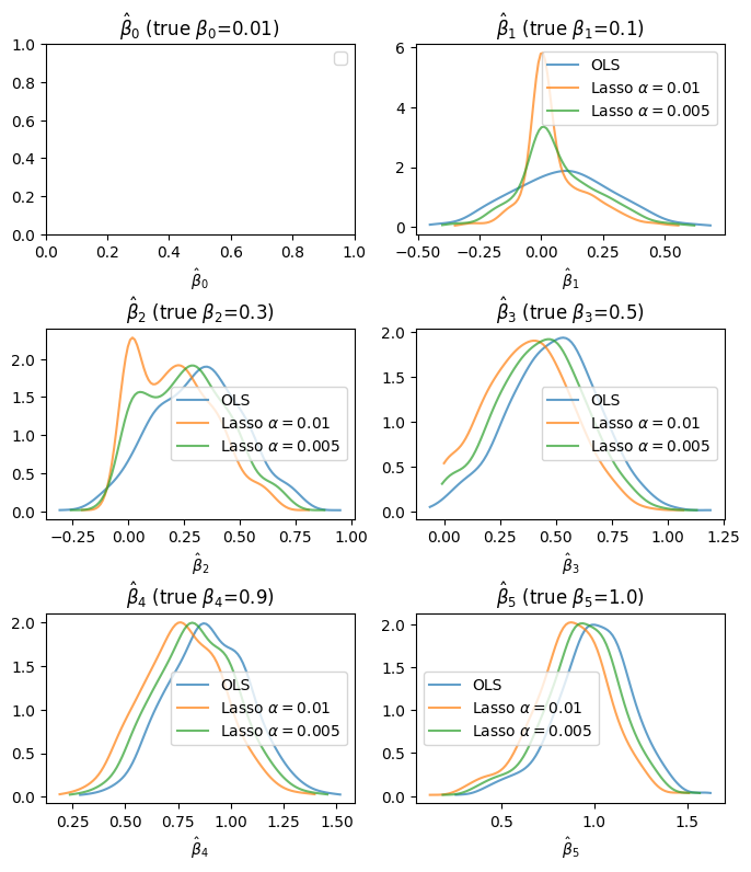
Lassoは正則化パラメータを強めにかけるとそのぶんバイアスは入る

import numpy as np
from sklearn.linear_model import Lasso, LinearRegression
from sklearn.metrics import mean_squared_error, r2_score
import matplotlib.pyplot as plt

true_coefs = np.array([0.01, 0.1, 0.3, 0.5, 0.9, 1])

def gen_data(n = 300, seed = 0):
    np.random.seed(seed)
    d = len(true_coefs)
    X = np.random.uniform(0, 1, size=(n, d))
    X[:, 0] = 1
    y = X @ true_coefs + np.random.normal(size=n, scale=1)
    return X, y


ols_coefs = []
alphas = [0.01, 0.005]
n_alpha = len(alphas)
lasso_coefs_list = []
for _ in range(n_alpha):
    lasso_coefs_list.append([])

n_trial = 500
for k in range(n_trial):
    X, y = gen_data(seed=k)

    for l in range(n_alpha):
        lasso = Lasso(alpha=alphas[l])
        lasso.fit(X, y)
        lasso_coefs_list[l].append(lasso.coef_)

    ols = LinearRegression()
    ols.fit(X, y)
    ols_coefs.append(ols.coef_)

for i in range(n_alpha):
    lasso_coefs_list[i] = np.array(lasso_coefs_list[i])
ols_coefs = np.array(ols_coefs)

n_features = ols_coefs.shape[1]
col_idx = 0
ncols = 2
nrows = int(np.ceil(n_features / ncols))

fig, axes = plt.subplots(figsize=[ncols * 4, nrows * 3], ncols=ncols, nrows=nrows)
fig.subplots_adjust(hspace=0.5)
axes = axes.flatten()
for col_idx in range(n_features):
    axes[col_idx].hist(ols_coefs[:, col_idx], bins=50, label="OLS", alpha=0.5)
    for l in range(n_alpha):
        lasso_coefs = lasso_coefs_list[l]
        axes[col_idx].hist(lasso_coefs[:, col_idx], bins=50, label=fr"Lasso $\alpha={alphas[l]}$", alpha=0.5)
    axes[col_idx].set(xlabel=fr"$\hat\beta_{col_idx}$", title=fr"$\hat\beta_{col_idx}$ (true $\beta_{col_idx}$={true_coefs[col_idx]})")
    axes[col_idx].legend()
# fig.suptitle(f"lasso alpha={alpha}")
fig.show()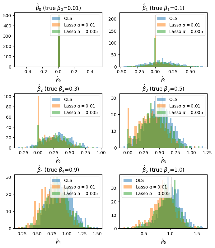

from scipy.stats import norm, gaussian_kde

def kdeplot(data, ax, label=None):
    try:
        kde = gaussian_kde(data)
        x = np.linspace(data.min(), data.max(), 100)
        y = kde.evaluate(x)
        ax.plot(x, y, label=label, alpha=0.7)
    except:
        pass
    return ax

n_features = ols_coefs.shape[1]
col_idx = 0
ncols = 2
nrows = int(np.ceil(n_features / ncols))

fig, axes = plt.subplots(figsize=[ncols * 4, nrows * 3], ncols=ncols, nrows=nrows)
fig.subplots_adjust(hspace=0.5)
axes = axes.flatten()
for col_idx in range(n_features):
    kdeplot(ols_coefs[:, col_idx], ax=axes[col_idx], label="OLS")
    for l in range(n_alpha):
        lasso_coefs = lasso_coefs_list[l]
        kdeplot(lasso_coefs[:, col_idx], ax=axes[col_idx], label=fr"Lasso $\alpha={alphas[l]}$")

    axes[col_idx].set(xlabel=fr"$\hat\beta_{col_idx}$", title=fr"$\hat\beta_{col_idx}$ (true $\beta_{col_idx}$={true_coefs[col_idx]})")
    axes[col_idx].legend()
# fig.suptitle(f"lasso alpha={alpha}")
fig.show()

No artists with labels found to put in legend.  Note that artists whose label start with an underscore are ignored when legend() is called with no argument.