分位点回帰 - データサイエンス関連+αのメモ

分位点 $\tau$ における条件付分位関数を

Q_\tau(y_i | X_i) = F_y^{-1}(\tau | X_i)

(1)

と表す。ここで $F_y^{-1}(\tau | X_i)$ は $y$ において $X_i$ に条件づけられた $y_i$ の分布関数である（ $F_y^{-1}(\tau | X_i) = \inf \{ y: F_y(y|X_i) \geq \tau \}$ ）。

例えば $\tau = 0.1$ のとき、 $Q_\tau(y_i | X_i)$ は $y_i$ の下位10分位である。

標準的な回帰モデルは二乗誤差 $(y_i - m(X_i))^2$ の和や期待値を最小化するようにモデル $m(X_i)$ を学習して条件付き期待値 $E(y_i|X_i)$ を予測する

\newcommand{\argmin} attempting to redefine \argmin; use \renewcommand

\newcommand{\argmin}{\mathop{\rm arg~min}\limits}
E(y_i|X_i) = \argmin_{m(X_i)}
E\big[ (y_i - m(X_i))^2 \big]

分位点回帰 （quantile regression）モデルはpinball loss $\rho_{\tau}(y_i - q(X_i))$ の和や期待値を最小化するようにモデル $q(X_i)$ を学習させ、条件付き分位関数 $Q_{\tau}(y_i|X_i) = F^{-1}_y(\tau|X_i)$ を予測する

Q_{\tau}(y_i|X_i) = \argmin_{q(X_i)} E\big[ \rho_{\tau}(y_i - q(X_i)) \big]

(3)

pinball lossは $\tau$ -tiled absolute value function や検定関数（check function）とも呼ばれる（グラフを描くとチェックマークに似てるため）

\rho_{\tau} (x) = \big(\tau - \mathbb{1}(x \leq 0) \big) x

(4)

あるいは

\rho_{\tau} (x) = \begin{cases} (\tau - 1) x & \text{ if } x \leq 0\\ \tau x & \text{ if } x > 0\\ \end{cases}

(5)

あるいは

\rho_{\tau} (x) = \tau \max(x, 0) + (\tau - 1) \min(-x, 0)

(6)

と書かれる

import numpy as np
import matplotlib.pyplot as plt

def pinball_loss(x, tau):
    return (tau - 1 * (x <= 0)) * x

x = np.linspace(-1, 1, 100)
fig, axes = plt.subplots(figsize=[10, 2], ncols=3)
for i, tau in enumerate([0.1, 0.5, 0.9]):
    y = pinball_loss(x, tau=tau)
    axes[i].plot(x, y)
    if i == 0:
        axes[i].set(title=f"τ={tau}", xlabel=r"$x$", ylabel=r"$y = (\tau - 1(x <= 0)) x$")
    else:
        axes[i].set(title=f"τ={tau}", xlabel=r"$x$")
fig.show()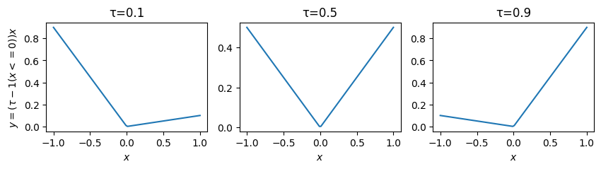

なお、pinball lossは $\tau=0.5$ のとき

\begin{align} \rho_{0.5} (x) &= \begin{cases} -0.5 x & \text{ if } x \leq 0\\ 0.5 x & \text{ if } x > 0\\ \end{cases} \\ &= \frac{1}{2} |x| \end{align}

(11)

と、絶対誤差と比例する形になる。

絶対誤差の和を目的関数にとった線形モデルは統計学においてleast absolute deviations (LAD) と呼ばれ、その解は条件付き中央値になる

\text{median}(y_i|X_i) = Q_{0.5}(y_i|X_i) = \argmin_{q(X_i)} E\big[ \rho_{0.5}(y_i - q(X_i)) \big]

(12)

import numpy as np
import matplotlib.pyplot as plt

def pinball_loss(x, tau):
    return (tau - 1 * (x <= 0)) * x

x = np.linspace(-3, 3, 100)
fig, ax = plt.subplots(figsize=[4, 3])
ax.plot(x, pinball_loss(x, tau=0.5), label=r"$\rho_{0.5}(x)$")
ax.plot(x, abs(x), label="|x|")
ax.legend()
fig.show()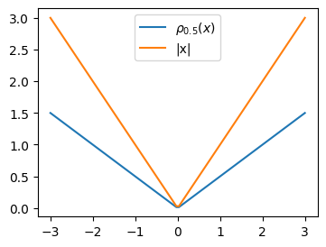

分位点回帰モデルの実践¶

LightGBMでのquantile regression¶

目的関数をbinball lossにすればいいだけなので他のアルゴリズムでも実行できる

import numpy as np
import matplotlib.pyplot as plt

# create data
np.random.seed(0)
n = 1000
x = np.random.uniform(-3, 3, size=n)
X = x.reshape(-1, 1)
y = np.sin(x) + np.random.normal(scale=0.5, size=n)

fig, ax = plt.subplots()
ax.scatter(x, y, alpha=0.7)

# regression
x_plot = np.linspace(-3, 3, 500)
X_test = x_plot.reshape(-1, 1)
import lightgbm as lgb
taus = [0.1, 0.9]
colors = ["orange", "tomato"]
for i in range(2):
    model = lgb.LGBMRegressor(objective="quantile", alpha=taus[i], verbose=-1)
    model.fit(X, y)
    y_hat = model.predict(X_test)
    ax.plot(X_test, y_hat, color=colors[i], label=fr"$\tau = {taus[i]}$")
ax.set(xlabel="x", ylabel="y", title="Quantile Regression with LightGBM")
ax.legend()
fig.show()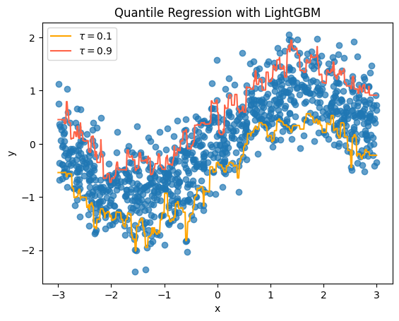

from sklearn.metrics import d2_pinball_score, make_scorer
d2_pinball_score_09 = make_scorer(d2_pinball_score, alpha=0.9)
d2_pinball_score_09(model, X, y)

0.48475107952573926