Source
import numpy as np
from scipy.stats import norm
import matplotlib.pyplot as plt

# gen data
# 2つの正規分布の混合分布
w = 0.3
params = [dict(loc=0.25, scale=0.1), dict(loc=0.75, scale=0.1)]

def pdf(x):
    return w * norm.pdf(x, **params[0]) + (1 - w) * norm.pdf(x, **params[1])


def rvs(size):
    n = int(w * size)
    return np.append(norm.rvs(size=n, random_state=0, **params[0]), norm.rvs(size=(size - n), random_state=0, **params[1]))


fig, axes = plt.subplots(figsize=[10, 3], ncols=2)
axes[0].set(xlabel="x", ylabel="probability density", title="probability density function")
x_range = np.linspace(0, 1, 100)
axes[0].plot(x_range, [pdf(xi) for xi in x_range], color="dimgray")

axes[1].set(xlabel="x", ylabel="count", title="histogram")
n = 50
x = rvs(n)
x = np.sort(x)
axes[1].hist(x, color="dimgray")
fig.show()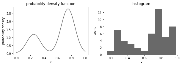
ヒストグラム密度推定法
ヒストグラム密度推定法(histogram density estimation method)
1つの連続変数が対象の場合を考える。
標準的なヒストグラムでは、を幅の区間に区切り、番目の区間に入ったの観測値の数と観測値の総数を用いて、各区間の確率密度を
で推定する。
Source
class HistogramEstimator:

    def __init__(self, bandwidth: float):
        self.h = bandwidth

    def fit(self, x: np.array):
        # calc bins
        range_ = max(x) - min(x)
        times = int(np.ceil(range_ / self.h))
        bins = [min(x) + self.h * i for i in range(times + 1)]
        # calc probabilities
        N = x.shape[0]
        probs = []
        deltas = []
        for i in range(1, len(bins)):
            values = x[(bins[i - 1] <= x) & (x < bins[i])]
            n = len(values)
            delta = bins[i] - bins[i - 1]
            p = n / (N * delta)
            probs.append(p)
            deltas.append((bins[i - 1], bins[i]))
        self.probs_ = probs
        self.deltas_ = deltas
        return self

    def score(self, x: np.array) -> np.array:
        p_pred = np.zeros(shape=x.shape[0])
        for (lower, upper), p in zip(self.deltas_, self.probs_):
            p_pred[(lower <= x) & (x < upper)] = p
        return p_pred

# plot
fig, axes = plt.subplots(figsize=[14, 3], ncols=3)

for ax, h in zip(axes, [0.05, 0.10, 0.2]):
    # true
    x_range = np.linspace(0, 1, 100)
    ax.plot(x_range, [pdf(xi) for xi in x_range], color="dimgray", label="True PDF")

    # estimates
    estimator = HistogramEstimator(bandwidth=h)
    estimator.fit(x)
    for (lower, upper), p in zip(estimator.deltas_, estimator.probs_):
        ax.bar(lower, p, h, color="white", edgecolor="steelblue")

    ax.bar(lower, p, h, color="white", edgecolor="steelblue", label="histogram method")

    ax.scatter(x, np.zeros(x.shape[0]), label="samples", color="gray", alpha=0.5)
    ax.set(xlabel="x", ylabel="probability density", title=f"Histogram method (h={h})")
    ax.legend()

fig.show()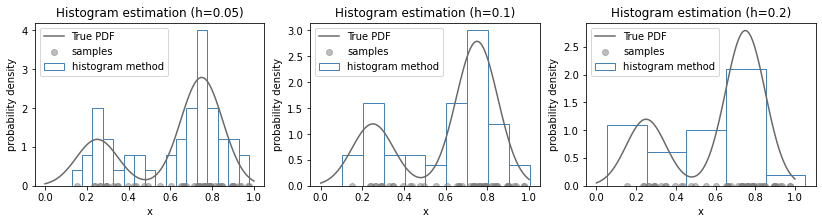
この方法の結果の良し悪しは区間幅に大きく依存する。幅が狭すぎても区間に含まれるサンプルが少なすぎて推定のばらつきが大きくなるし、幅が広すぎても表現力が不足して分布をうまく捉えられなくなる。
また、ヒストグラム法の問題として
推定した密度が区間の縁で不連続になる
次元の呪いに弱い:次元数を上げていった場合、次元空間を各変数につき個の区間にすると、区間の総数は個になり、各区間に含まれるデータ量が不足する
といったものがある
カーネル密度推定法
次元のユークリッド空間中の未知の確率密度から観測値の集合が得られていて、この集合からの値を推定したいとする。
を含むある小さな領域を考える。この領域に割り当てられた確率は
と表すことができる。
glue:figure - Unknown Directive
glue:figure - Unknown Directive:figwidth: 80% :name: "fig-region"
大きいについては、分散が小さくなって平均の周囲で鋭く尖った分布となり、
となる。
が確率密度がこの領域内でほぼ一定とみなせるほど十分に小さいものであると仮定できるのであれば、領域の体積を用いて
となる。
これらを組み合わせて、次の密度の推定量が得られる。
カーネル関数
確率密度を求めたいデータ点を中心とする小さな超立方体を領域とする。 この領域内にある点の数を数えるには、次の関数を定義しておくと便利である。
これは原点を中心とする単位立方体を表す。 関数はカーネル関数(kernel function)のひとつであり、今回の用途ではParzen窓(parzen window)とも呼ばれる。
Source
def k(u):
    return 1 * all([abs(ui) <= (1/2) for ui in u])

u1 = np.linspace(-1, 1, 51)
u2 = np.linspace(-1, 1, 51)
u1, u2 = np.meshgrid(u1, u2)
k_ = np.array([k([_u1, _u2]) for _u1, _u2 in zip(u1.flatten(), u2.flatten())]).reshape(u1.shape)

fig, ax = plt.subplots(dpi=100, subplot_kw={"projection": "3d"})
ax.plot_surface(u1, u2, k_, rstride=1, cstride=1, linewidth=1, antialiased=True, alpha=0.7)
ax.set(xlabel="u1", ylabel="u2", zlabel="k", title="k(u)", zlim=[0, 2])
fig.show()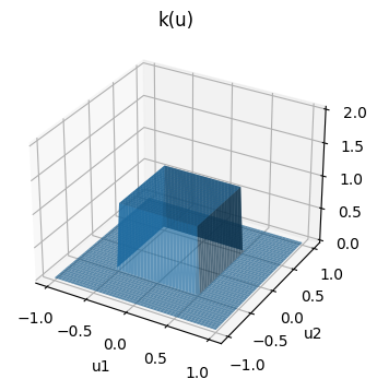
はを中心とする一辺がの立方体の内部に、データ点があれば1に、そうでなければ0となる。
例えばの場合は次の図のようになる
Source
_x = np.array([2, 3])
h = 2

x1 = np.linspace(-1, 5, 51)
x2 = np.linspace(0, 5, 51)
x1, x2 = np.meshgrid(x1, x2)
k_ = np.array([k( ( _x - np.array([_x1, _x2]) ) / h )
               for _x1, _x2 in zip(x1.flatten(), x2.flatten())]).reshape(u1.shape)

fig, ax = plt.subplots(dpi=100, subplot_kw={"projection": "3d"})

ax.scatter(_x[0], _x[1], color="orange")
ax.text(_x[0] * 1.1, _x[1] * 1.1, 0, f"x=({_x[0]}, {_x[1]})", color="orange")

ax.plot_surface(x1, x2, k_, rstride=1, cstride=1, linewidth=1, antialiased=True, alpha=0.4)
ax.set(xlabel="x1", ylabel="x2", zlabel="k", title="k([x - x_n] / h)", zlim=[0, 2.5])
fig.show()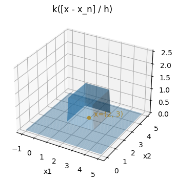
このカーネルを使用した推定結果は次の図のようになる。 立方体を重ねるような推定を行うため平滑性がなく、ギザギザした密度関数が推定されている。
Source
class KernelEstimator:

    def __init__(self, bandwidth: float):
        self.h = bandwidth

    def fit(self, X: np.array):
        self.X_train_ = X
        self.N_ = X.shape[0]
        self.D_ = X.shape[1]
        return self

    def score(self, X: np.array) -> np.array:
        p_preds = []
        for x in X:
            U = (x - self.X_train_) / self.h
            K = [k(u) for u in U]
            p_pred = (1 / self.N_) * (1 / self.h ** self.D_) * np.sum( K )
            p_preds.append(p_pred)
        return np.array(p_preds)

# plot
fig, axes = plt.subplots(figsize=[14, 3], ncols=3)

for ax, h in zip(axes, [0.05, 0.10, 0.20]):
    # true
    x_range = np.linspace(0, 1, 100)
    ax.plot(x_range, [pdf(xi) for xi in x_range], color="dimgray", label="True PDF")

    # estimates
    X_train = x.reshape(-1, 1)
    X_test = x_range.reshape(-1, 1)

    estimator = KernelEstimator(bandwidth=h)
    estimator.fit(X_train)
    p = estimator.score(X_test)
    ax.plot(x_range, p, label="estimated PDF")

    ax.scatter(x, np.zeros(x.shape[0]), label="samples", color="gray", alpha=0.5)
    ax.set(xlabel="x", ylabel="probability density", title=f"Kernel method (h={h})")
    ax.legend()

fig.show()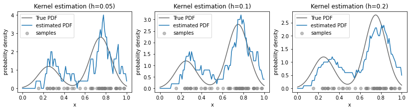
Source
from scipy.stats import norm

class GaussianKernelEstimator:

    def __init__(self, bandwidth: float):
        self.h = bandwidth

    def fit(self, X: np.array):
        self.X_train_ = X
        self.N_ = X.shape[0]
        self.D_ = X.shape[1]
        return self

    def score(self, X: np.array) -> np.array:
        p_preds = []
        for x in X:
            p_pred = norm.pdf(x=x, loc=self.X_train_, scale=self.h).mean()
            p_preds.append(p_pred)
        return np.array(p_preds)

# plot
fig, axes = plt.subplots(figsize=[14, 3], ncols=3)

for ax, h in zip(axes, [0.02, 0.05, 0.10]):
    # true
    x_range = np.linspace(0, 1, 100)
    ax.plot(x_range, [pdf(xi) for xi in x_range], color="dimgray", label="True PDF")

    # estimates
    X_train = x.reshape(-1, 1)
    X_test = x_range.reshape(-1, 1)

    estimator = GaussianKernelEstimator(bandwidth=h)
    estimator.fit(X_train)
    p = estimator.score(X_test)
    ax.plot(x_range, p, label="estimated PDF")

    ax.scatter(x, np.zeros(x.shape[0]), label="samples", color="gray", alpha=0.5)
    ax.set(xlabel="x", ylabel="probability density", title=f"Gaussian Kernel method (h={h})")
    ax.legend()

fig.show()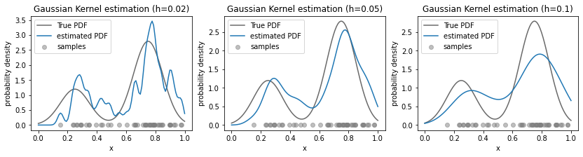
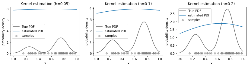
Source
# 数式からガウスカーネルを実装したけど合わなかったやつ
def gauss(x, x_n, h, D):
    y = (1 / (2 * np.pi * h **2)**(D/2)) * np.exp(-(np.linalg.norm(x - x_n)**2 / 2 * h ** 2))
    return np.mean(y)

class GaussianKernelEstimator:

    def __init__(self, bandwidth: float):
        self.h = bandwidth

    def fit(self, X: np.array):
        self.X_train_ = X
        self.N_ = X.shape[0]
        self.D_ = X.shape[1]
        return self

    def score(self, X: np.array) -> np.array:
        p_preds = []
        for x in X:
            p_pred = gauss(x, x_n=self.X_train_, h=self.h, D=self.D_)
            p_preds.append(p_pred)
        return np.array(p_preds)

# plot
fig, axes = plt.subplots(figsize=[14, 3], ncols=3)

for ax, h in zip(axes, [0.05, 0.10, 0.20]):
    # true
    x_range = np.linspace(0, 1, 100)
    ax.plot(x_range, [pdf(xi) for xi in x_range], color="dimgray", label="True PDF")

    # estimates
    X_train = x.reshape(-1, 1)
    X_test = x_range.reshape(-1, 1)

    estimator = GaussianKernelEstimator(bandwidth=h)
    estimator.fit(X_train)
    p = estimator.score(X_test)
    ax.plot(x_range, p, label="estimated PDF")

    ax.scatter(x, np.zeros(x.shape[0]), label="samples", color="gray", alpha=0.5)
    ax.set(xlabel="x", ylabel="probability density", title=f"Kernel method (h={h})")
    ax.legend()

fig.show()
Output
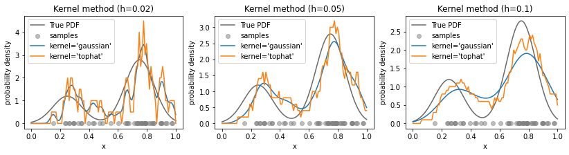
(参考)Scikit-learn実装
2.8. Density Estimation — scikit-learn 1.2.2 documentation
(※kernel='tophat'は立方体カーネルに近い というもの)
Source
from sklearn.neighbors import KernelDensity

fig, axes = plt.subplots(figsize=[14, 3], ncols=3)
for ax, h in zip(axes, [0.02, 0.05, 0.10]):
    # true
    x_range = np.linspace(0, 1, 100)
    ax.plot(x_range, [pdf(xi) for xi in x_range], color="dimgray", label="True PDF")
    ax.scatter(x, np.zeros(x.shape[0]), label="samples", color="gray", alpha=0.5)

    # estimates
    X_train = x.reshape(-1, 1)
    X_test = x_range.reshape(-1, 1)

    for method in ["gaussian", "tophat"]:
        kde = KernelDensity(kernel=method, bandwidth=h).fit(X_train)
        log_likelihood = kde.score_samples(X_test)
        ax.plot(x_range, np.exp(log_likelihood), label=f"kernel='{method}'")
    ax.set(xlabel="x", ylabel="probability density", title=f"Kernel method (h={h})")
    ax.legend()
fig.show()