サンプルサイズの決め方

区間推定のサンプルサイズの決め方¶

信頼区間の幅を基準にサンプルサイズを決める方法がある。

母比率 $p$ の95%信頼区間は、標本比率 $\hat{p}$ を用いて

\widehat{p}-1.96 \times \sqrt{\frac{\widehat{p}(1-\widehat{p})}{n}} \leq p \leq \widehat{p}+1.96 \times \sqrt{\frac{\widehat{p}(1-\widehat{p})}{n}}

(1)

と求めることができる

区間の幅部分が両側合計で $w$ 以下にしたい場合は

2 \times 1.96 \times \sqrt{\frac{\widehat{p}(1-\widehat{p})}{n}} \leq w

(2)

を解けばよいので

\sqrt{n} \geq 2 \times 1.96 \times \sqrt{\widehat{p}(1-\widehat{p})} \times \frac{1}{w}

(3)

n \geq (2 \times 1.96 \times \sqrt{\widehat{p}(1-\widehat{p})} \times \frac{1}{w})^2

(4)

となる

例えば、事前調査により $\hat{p} = 0.1$ であることがわかっていて、幅 $w=0.01$ で95%信頼区間を求めたい場合は

from math import sqrt

w = 0.01
p_hat = 0.1

n = int( (2 * 1.96 * sqrt(p_hat * (1 - p_hat)) / w) ** 2 )
print(f"{n=}")

n=13829

# 信頼区間の計算
from scipy.stats import norm, sem

mu = p_hat
lower, upper = norm.interval(confidence=0.95, loc=mu, scale=sqrt((p_hat * (1 - p_hat)) / n))
width = (mu - lower) + (upper - mu)
print(f"[{lower:.3g}, {upper:.3g}], width={width:.1g}")

[0.095, 0.105], width=0.01

# 乱数生成してシミュレーション
import numpy as np
np.random.seed(0)
x = np.random.binomial(n=1, p=p_hat, size=int(n))

from scipy.stats import norm, sem
lower, upper = norm.interval(confidence=0.95, loc=x.mean(), scale=sem(x))
width = (x.mean() - lower) + (upper - x.mean())
print(f"[{lower:.3g}, {upper:.3g}], width={width:.1g}")

[0.0937, 0.104], width=0.01

statsmodelsの関数¶

samplesize_confint_proportion を使うことで、想定される比率、幅、有意水準からサンプル数を推定できる

from statsmodels.stats.proportion import samplesize_confint_proportion

n = samplesize_confint_proportion(proportion=0.1, half_length=0.01, alpha=0.05, method='normal')
print(f"{n:,.0f}")

3,457

参考

21-4. 必要なサンプルサイズ1 | 統計学の時間 | 統計WEB

検定のサンプルサイズの決め方（決定力分析）¶

検定は4つの要因で構成される

そこで、次の手順で

手順1. 事前分析：サンプルサイズの設計¶

調査（A/Bテストなど）を行う前のサンプルサイズ設計。

効果量
有意水準
検出力

を決めてサンプルサイズを算出する。

有意水準は5%、検出力は80%などにすればいいが、効果量がちょっと難しい。

A/Bテストでいうと「この新施策で成約率が5ポイント上昇するはず」などの仮定をおいて効果量を算出することになる。

効果量¶

代表的な効果量にはCohenのdやhがある。

効果量	用途	備考
Cohen’s $d$	2群の平均値の差	目安：0.2=小, 0.5=中, 0.8=大
Hedges’ $g$	2群の平均値の差	Cohen’s $d$ の小標本でのバイアス補正版
Cohen’s $h$	2群の比率の差	目安：0.2=小, 0.5=中, 0.8=大

import numpy as np

def cohens_d(x1: np.array, x2: np.array) -> float:
    n1, n2 = len(x1), len(x2)
    denom = (n1 - 1) * x1.std()**2 + (n2 - 1) * x2.std()**2
    num = n1 + n2 - 2
    pooled_std = np.sqrt(denom / num)
    return (x1.mean() - x2.mean()) / pooled_std

np.random.seed(0)

d = cohens_d(
    x1 = np.random.normal(loc=0, scale=1, size=450),
    x2 = np.random.normal(loc=0, scale=1, size=300),
)
print(f"{d=:.3f}")


d = cohens_d(
    x1 = np.random.normal(loc=0.5, scale=1, size=350),
    x2 = np.random.normal(loc=0, scale=1, size=300),
)
print(f"{d=:.3f}")

d=0.103
d=0.485

def hedges_g(x1: np.array, x2: np.array) -> float:
    d = cohens_d(x1, x2)
    n1, n2 = len(x1), len(x2)
    J = 1 - (3 / (4 * (n1 + n2 - 2) - 1))
    return J * d

np.random.seed(0)

x1 = np.random.normal(loc=0, scale=2, size=150)
x2 = np.random.normal(loc=0, scale=1, size=100)

d = cohens_d(x1, x2)
print(f"{d=:.3f}")
J = 1 - (3 / (4 * (x1.size + x2.size - 2) - 1))
print(f"{J=:.3f}")
g = hedges_g(x1, x2)
print(f"{g=:.3f}")

d=0.213
J=0.997
g=0.212

import math

def cohens_h(p1, p2):
    return 2 * (math.asin(p1**0.5) - math.asin(p2**0.5))

h = cohens_h(0.15, 0.10)
print(f"{h=:.3f}")

h=0.152

手順2. 事後分析：検出力の計算¶

実測のサンプルサイズ
実測の効果量
有意水準

で検出力を算出する

# 平均値の差の場合 ------------------------------
# サンプルの例
import numpy as np
np.random.seed(0)
x1 = np.random.normal(loc=0.2, scale=2, size=150)
x2 = np.random.normal(loc=0, scale=1, size=100)

# calc power
from statsmodels.stats.power import TTestIndPower
power_analysis = TTestIndPower()
power = power_analysis.power(
    nobs1=x1.size,
    ratio=x2.size / x1.size,  # nobs2 = nobs1 * ratio
    effect_size=hedges_g(x1, x2),
    alpha=0.05,
)
print(f"{power=:.3f}")

power=0.721

# 比率の差の場合 ------------------------------
# サンプルの例
import numpy as np
np.random.seed(0)
x1 = np.random.binomial(n=1, p=0.10, size=750)
x2 = np.random.binomial(n=1, p=0.15, size=600)

# calc power
from statsmodels.stats.power import NormalIndPower
power_analysis = NormalIndPower()
power = power_analysis.power(
    nobs1=x1.size,
    ratio=x2.size / x1.size,  # nobs2 = nobs1 * ratio
    effect_size=hedges_g(x1, x2),
    alpha=0.05,
)
print(f"{power=:.3f}")

power=0.954

statsmodels¶

statsmodels: Size Calculations

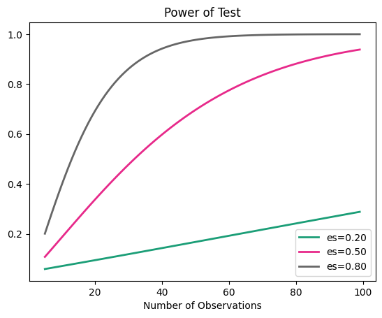
# サンプルサイズの変化に応じた検定力の推移
import numpy as np
from statsmodels.stats.power import TTestIndPower

power_analysis = TTestIndPower()
fig = power_analysis.plot_power(
    dep_var='nobs',
    nobs=np.arange(5, 100),
    effect_size=[0.2, 0.5, 0.8],
    alpha=0.05,
)

statsmodelsの solve_power では、4要因のうち None にした要素を推定できる

# effect_sizeをNoneにしてeffect_sizeを推定
from statsmodels.stats.power import TTestIndPower
power_analysis = TTestIndPower()
effect_size = power_analysis.solve_power(
    nobs1=100,
    ratio=1.0,  # nobs2 = nobs1 * ratio
    effect_size=None,
    alpha=0.05,
    power=0.80,
)
print(f"{effect_size=:.3f}")

effect_size=0.398

# effect_sizeをNoneにして必要なeffect_sizeを推定
from statsmodels.stats.power import NormalIndPower
power_analysis = NormalIndPower()
effect_size = power_analysis.solve_power(
    nobs1=1000,
    ratio=1.0,  # nobs2 = nobs1 * ratio
    effect_size=None,
    alpha=0.05,
    power=0.80,
)
print(f"{effect_size=:.3f}")

effect_size=0.125

区間推定のサンプルサイズの決め方¶

statsmodelsの関数¶

検定のサンプルサイズの決め方（決定力分析）¶

手順1. 事前分析：サンプルサイズの設計¶

効果量¶

手順2. 事後分析：検出力の計算¶

statsmodels¶

参考¶