評価指標 - データサイエンス関連+αのメモ

物体検出モデルの評価に使われる代表的な指標をまとめる。ここで扱うIoU・NMS・mAPは、Two-stage・One-stage・Anchor-free・Transformer系のいずれのパラダイムでも共通して使われる基礎的な概念。

IoU（Intersection over Union）¶

IoU（Intersection over Union、和集合に対する共通部分の割合） は、2つの矩形領域 $A, B$ がどれだけ重なっているかを表す指標。

\mathrm{IoU}(A, B) = \frac{|A \cap B|}{|A \cup B|}

(1)

$\mathrm{IoU} \in [0, 1]$ で、完全に一致すれば1、重なりがなければ0になる。物体検出では

予測ボックスと正解ボックスが「同じ物体を指しているか」の判定（例： $\mathrm{IoU} \geq 0.5$ なら正検出とみなす）
後述のNMSにおける重複ボックスの判定
後述のFaster R-CNNのアンカーへのラベル付け

など、検出パイプラインのあらゆる箇所で使われる最も基本的な指標。

import matplotlib.pyplot as plt
import matplotlib.patches as patches
import matplotlib_fontja
import numpy as np


def box_iou(box1, box2):
    # box = (x_min, y_min, x_max, y_max)
    xa = max(box1[0], box2[0])
    ya = max(box1[1], box2[1])
    xb = min(box1[2], box2[2])
    yb = min(box1[3], box2[3])

    inter_w = max(0.0, xb - xa)
    inter_h = max(0.0, yb - ya)
    inter_area = inter_w * inter_h

    area1 = (box1[2] - box1[0]) * (box1[3] - box1[1])
    area2 = (box2[2] - box2[0]) * (box2[3] - box2[1])
    union_area = area1 + area2 - inter_area

    return inter_area / union_area if union_area > 0 else 0.0


box_gt = (2, 2, 7, 7)
box_pred = (4, 3, 9, 8)
iou = box_iou(box_gt, box_pred)

fig, ax = plt.subplots(figsize=[4, 4])
ax.add_patch(patches.Rectangle((box_gt[0], box_gt[1]), box_gt[2] - box_gt[0], box_gt[3] - box_gt[1],
                                linewidth=2, edgecolor="tab:blue", facecolor="tab:blue", alpha=0.3, label="ground truth"))
ax.add_patch(patches.Rectangle((box_pred[0], box_pred[1]), box_pred[2] - box_pred[0], box_pred[3] - box_pred[1],
                                linewidth=2, edgecolor="tab:orange", facecolor="tab:orange", alpha=0.3, label="prediction"))
ax.set_xlim(0, 10)
ax.set_ylim(0, 10)
ax.set_aspect("equal")
ax.set_title(f"IoU = {iou:.3f}")
ax.legend(loc="upper left")
plt.show()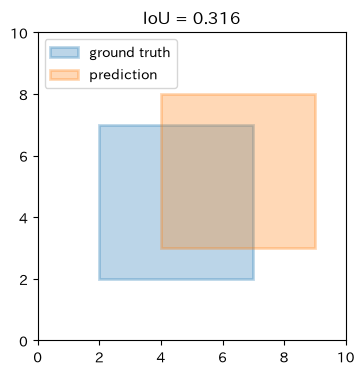

NMS（Non-Maximum Suppression）¶

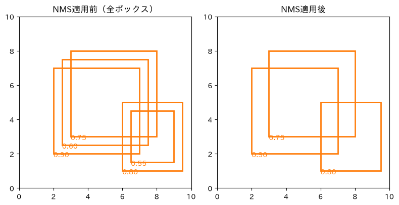
物体検出モデルは通常、1つの物体に対して多数の重複したボックスを予測する（後述のスライディングウィンドウ／アンカー／グリッドベースの手法では特に顕著）。NMS（Non-Maximum Suppression、非最大値抑制） は、この重複した検出結果から最も確からしい1つだけを残すための後処理アルゴリズム。

アルゴリズム

検出結果を信頼度スコア $s_i$ の降順に並べる
最もスコアが高いボックス $b$ を採用し、出力集合に加える
残りのボックスのうち、 $b$ とのIoUが閾値 $\tau$ 以上のもの（＝ $b$ と同じ物体を指していると判断されるもの）を除去する
残ったボックスに対して2〜3を繰り返す

$\tau$ （典型的には 0.5 程度）は、どこまでの重なりを「同じ物体」とみなすかを決めるハイパーパラメータ。

def nms(boxes, scores, iou_threshold=0.5):
    order = np.argsort(scores)[::-1]
    keep = []
    while len(order) > 0:
        i = order[0]
        keep.append(i)
        rest = order[1:]
        ious = np.array([box_iou(boxes[i], boxes[j]) for j in rest])
        order = rest[ious < iou_threshold]
    return keep


rng = np.random.default_rng(0)
boxes = np.array([
    [2, 2, 7, 7],
    [3, 3, 8, 8],
    [2.5, 2.5, 7.5, 7.5],
    [6, 1, 9.5, 5],
    [6.5, 1.5, 9, 4.5],
])
scores = np.array([0.9, 0.75, 0.6, 0.8, 0.55])

keep = nms(boxes, scores, iou_threshold=0.5)
print("keep indices:", keep)

fig, axes = plt.subplots(1, 2, figsize=[8, 4])
titles = ["NMS適用前（全ボックス）", "NMS適用後"]
for ax, idx, title in zip(axes, [range(len(boxes)), keep], titles):
    for i in idx:
        ax.add_patch(patches.Rectangle((boxes[i, 0], boxes[i, 1]), boxes[i, 2] - boxes[i, 0], boxes[i, 3] - boxes[i, 1],
                                        linewidth=2, edgecolor="tab:orange", facecolor="none"))
        ax.text(boxes[i, 0], boxes[i, 1] - 0.2, f"{scores[i]:.2f}", color="tab:orange")
    ax.set_xlim(0, 10)
    ax.set_ylim(0, 10)
    ax.set_aspect("equal")
    ax.set_title(title)
plt.tight_layout()
plt.show()

keep indices: [np.int64(0), np.int64(3), np.int64(1)]

mAP（mean Average Precision）¶

物体検出モデルの精度を単一の数値で比較するための指標。以下の順に定義していく。

適合率と再現率

IoUがある閾値以上（例：0.5）の予測を正検出（True Positive, TP）、そうでない予測を誤検出（False Positive, FP）、検出できなかった正解を検出漏れ（False Negative, FN）として、

\mathrm{Precision} = \frac{TP}{TP + FP}, \qquad \mathrm{Recall} = \frac{TP}{TP + FN}

(2)

Average Precision（AP）

信頼度スコアの閾値を変化させながら（＝スコアの高い予測から順に採用していきながら）Precision-Recall曲線を描き、その曲線の下側面積として1クラス分のAPを定義する。

\mathrm{AP} = \int_0^1 p(r)\, dr

(3)

実務上は、Recallを一定間隔（PASCAL VOC以前は11点、それ以降は全点）でサンプリングし、各Recall水準以上でのPrecisionの最大値（interpolated precision）を積分近似することが多い。

mAP

\mathrm{mAP} = \frac{1}{|C|} \sum_{c \in C} \mathrm{AP}_c

(4)

全クラス $C$ にわたってAPを平均したものがmAP。代表的なベンチマークでの定義の違い：

ベンチマーク	mAPの定義
PASCAL VOC	IoU閾値 0.5 における mAP（ $\mathrm{mAP}@0.5$ ）
MS COCO	IoU閾値 0.5〜0.95 を 0.05 刻みで変化させた mAP の平均（ $\mathrm{mAP}@[.5:.95]$ ）

COCOのmAPはIoU閾値を厳しくしたケースも平均に含めるため、ボックスの位置精度もより強く評価される。

# トイデータでPrecision-Recall曲線とAPを計算する例
# 1クラス・1画像に対する検出結果（スコア降順）と、正検出(1)/誤検出(0)のラベル
scores_toy = np.array([0.95, 0.9, 0.8, 0.7, 0.6, 0.5, 0.4, 0.3])
is_tp = np.array([1, 1, 0, 1, 0, 1, 0, 0])  # IoU>=0.5で正解と対応付けられたか
n_gt = 5  # この画像・クラスにおける正解ボックスの総数

tp_cum = np.cumsum(is_tp)
fp_cum = np.cumsum(1 - is_tp)
precision = tp_cum / (tp_cum + fp_cum)
recall = tp_cum / n_gt

# interpolated precision: 各recall水準でそれ以降のprecisionの最大値をとる
precision_interp = np.maximum.accumulate(precision[::-1])[::-1]

# 台形則ではなく、recallが変化した点でのprecisionを足し合わせる形でAPを近似
recall_padded = np.concatenate([[0], recall])
ap = np.sum((recall_padded[1:] - recall_padded[:-1]) * precision_interp)

fig, ax = plt.subplots(figsize=[5, 4])
ax.step(recall, precision, where="post", label="precision", color="tab:blue")
ax.step(recall, precision_interp, where="post", label="interpolated precision", color="tab:orange", linestyle="--")
ax.set_xlabel("Recall")
ax.set_ylabel("Precision")
ax.set_xlim(0, 1)
ax.set_ylim(0, 1.05)
ax.set_title(f"AP = {ap:.3f}")
ax.legend()
plt.show()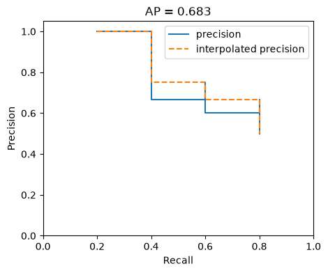

参考文献¶

Mean Average Precision (mAP) Explained | Paperspace Blog
IoU (Intersection over Union) for object detection - PyImageSearch
Everingham, M. et al. (2010). The PASCAL Visual Object Classes (VOC) Challenge
Lin, T.-Y. et al. (2014). Microsoft COCO: Common Objects in Context

References¶

Everingham, M., Van Gool, L., Williams, C. K. I., Winn, J., & Zisserman, A. (2009). The Pascal Visual Object Classes (VOC) Challenge. International Journal of Computer Vision, 88(2), 303–338. 10.1007/s11263-009-0275-4