概要
一般化部分得点モデル(Generalized Partial Credit Model: GPCM, Muraki, 1992) は多値の順序尺度の反応を扱えるIRTモデル。
GRMとGPCMの使い分けについて
SATの実世界データとシミュレーションデータを使ってGPCMとGRMを比較した。
の推定値は相関係数 0.9748 ~ 0.9921と高い相関を示した。
データ:Rの
irtplayパッケージのsimdat()関数で、GRMとGPCMの下でのデータを生成。異なるサンプルサイズ・項目数・欠損率で比較。GRM生成データをGPCMで分析すると収束しないケースが多い→やはり両モデルは若干異なる
項目母数の安定性:GPCM > GRM
能力母数の精度:GRM > GPCM(ただし高欠測率の時はGPCMが安定)
テスト情報量はGRMが高くなる傾向がある
考え方
隣のカテゴリとの2択で考える
2カテゴリの場合
とする。2PLモデルにおいては、
「の確率(カテゴリ0を選ぶ確率)」と「の確率(カテゴリ1を選ぶ確率)」の合計は1になる。そして「カテゴリ1を選ぶ確率」は
と表すことができる。
カテゴリの場合
これをカテゴリ()に一般化し、「隣り合う2つのカテゴリとの二択においてを選ぶ確率」とする。
これは反応 が か のどちらかだと仮定して正規化したとき、 が選ばれる「相対的な割合」。
式を
の形に変形すると
となる。
漸化式の形に変形
ここで、とのカテゴリの2択であるということで、2PLMと同様にロジスティックモデルで表現できるとすると、
と対数オッズを線形モデルで表現する形に表すことができる。この両辺に指数をとると
になる。簡単のためとすると、式は
という漸化式の形になる。言葉で書くと、「特定のカテゴリを選ぶ確率 」は、「 を選ぶ確率 」と「隣のカテゴリに移るオッズ 」で表すことができるというもの。
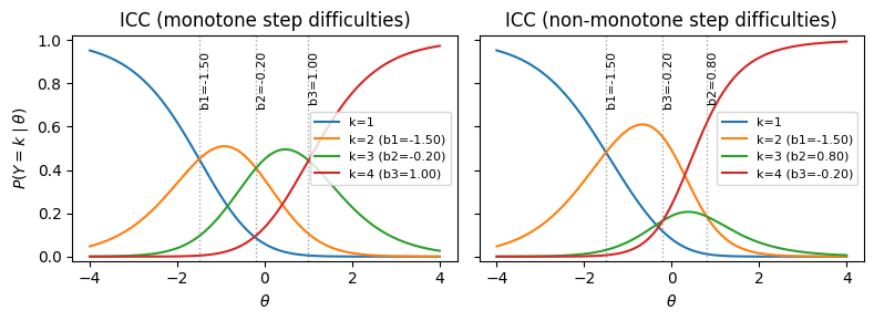
例えば3カテゴリの場合は
のようになる。つまり、にの積を掛け合わせた形ですべてのカテゴリの反応確率が表される。
いったんとして、 を代入すると
Source
import numpy as np
import matplotlib.pyplot as plt

def gpcm_probs(theta, a, b_steps):
    """
    theta: shape (T,)
    a: float
    b_steps: shape (K-1,)
    returns: P shape (T, K)
    """
    theta = np.asarray(theta)
    b_steps = np.asarray(b_steps)

    K = b_steps.size + 1

    inc = a * (theta[:, None] - b_steps[None, :])  # (T, K-1)
    csum = np.cumsum(inc, axis=1)                  # (T, K-1)

    log_num = np.concatenate(
        [np.zeros((theta.size, 1)), csum],
        axis=1
    )  # (T, K)

    mx = np.max(log_num, axis=1, keepdims=True)
    exp_shift = np.exp(log_num - mx)
    P = exp_shift / np.sum(exp_shift, axis=1, keepdims=True)

    return P

# example ----------------------------------
theta = np.linspace(-4, 4, 801)
a = 1.2
K = 4

# --- ケース1:困難度が単調増加 ---
b_mono = np.array([-1.5, -0.2, 1.0])
P_mono = gpcm_probs(theta, a, b_mono)

# --- ケース2:困難度が非単調 ---
b_nonmono = np.array([-1.5, 0.8, -0.2])
P_nonmono = gpcm_probs(theta, a, b_nonmono)

fig, axes = plt.subplots(ncols=2, figsize=(8, 3), sharey=True)

# 共通設定
y_text = 0.95   # テキストの y 位置(確率スケール)
text_kwargs = dict(rotation=90, va="top", ha="left", fontsize=8)

# -----------------------------
# 左:単調増加
# -----------------------------
ax = axes[0]
for k in range(K):
    if k == 0:
        label = "k=1"
    else:
        label = f"k={k+1} (b{k}={b_mono[k-1]:.2f})"
    ax.plot(theta, P_mono[:, k], label=label)

# 縦線 + 注記(k=2..K に対応する b)
for i, b in enumerate(b_mono, start=1):
    ax.axvline(b, linestyle=":", linewidth=1, alpha=0.7, color="gray")
    ax.text(b, y_text, f"b{i}={b:.2f}", **text_kwargs)

ax.set_ylim(-0.02, 1.02)
ax.set_xlabel(r"$\theta$")
ax.set_ylabel(r"$P(Y=k\mid\theta)$")
ax.set_title("ICC (monotone step difficulties)")
ax.legend(fontsize=8, loc="right")

# -----------------------------
# 右:非単調
# -----------------------------
ax = axes[1]
for k in range(K):
    if k == 0:
        label = "k=1"
    else:
        label = f"k={k+1} (b{k}={b_nonmono[k-1]:.2f})"
    ax.plot(theta, P_nonmono[:, k], label=label)

# 縦線 + 注記
for i, b in enumerate(b_nonmono, start=1):
    ax.axvline(b, linestyle=":", linewidth=1, alpha=0.7, color="gray")
    ax.text(b, y_text, f"b{i}={b:.2f}", **text_kwargs)

ax.set_ylim(-0.02, 1.02)
ax.set_xlabel(r"$\theta$")
ax.set_title("ICC (non-monotone step difficulties)")
ax.legend(fontsize=8)

plt.tight_layout()
plt.show()
# ESC(単調ケース)
E_mono = np.sum((np.arange(1, K+1)[None, :]) * P_mono, axis=1)

# ESC(非単調ケース)
E_nonmono = np.sum((np.arange(1, K+1)[None, :]) * P_nonmono, axis=1)

plt.figure(figsize=(5, 3))
plt.plot(theta, E_mono, label="monotone b")
plt.plot(theta, E_nonmono, linestyle="--", label="non-monotone b")

plt.xlabel(r"$\theta$")
plt.ylabel(r"$\mathbb{E}[Y\mid\theta]$")
plt.title("Expected Score Curve (ESC)")
plt.legend()
plt.tight_layout()
plt.show()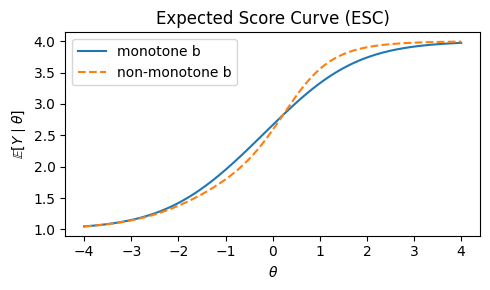
部分得点モデル
部分得点モデル(Partial Credit Model: PCM, Masters, 1982) は Raschモデルを順序多値に拡張した IRT モデル。
あるいはロジットで表すと
PCMでは識別力パラメータは 存在しない(全部共通で)ため扱いにくく、一般化したGPCMが提案された
一般化部分得点モデル
一般化部分得点モデル(Generalized Partial Credit Model: GPCM, Muraki, 1992) はPCMを一般化し、項目ごとに異なる識別力を導入したモデル。
あるいは
:項目 の識別力
:段階 の難易度
実装
最尤推定ならRのmirtパッケージでgpcmを選ぶだけだが、ベイズモデリングはややこしい
BUGS
1	model {
2	    for (i in 1:n) {
3	        for (j in 1:p) {
4	                Y[i, j] ~ dcat(prob[i, j, 1:K[j]])
5	                }
6	                theta[i] ~ dnorm(mu0, tau0)
7	    }
8	    for (i in 1:n) {
9	        for (j in 1:p) {
10	            for (k in 1:K[j] ) {
11	                eta[i, j, k] <- alpha[j] * (theta[i] - beta[j, k])
12	                psum[i, j, k] <- sum(eta[i, j, 1:k])
13	                exp.psum[i, j, k] <- exp(psum[i, j, k])
14	                prob[i, j, k] <- exp.psum[i, j, k] / sum(exp.psum[i, j, 1:K[j]])
15	    } } }
16	    for (j in 1:p) {
17	        alpha[j] ~ dlnorm(m.alpha, pr.alpha)
18	        beta[j, 1] <- 0.0
19	        for (k in 2:K[j]) {
20	                beta[j, k] ~ dnorm(m.beta, pr.beta)
21	        }
22	    }
23	    pr.alpha <- pow(s.alpha, −2)
24	    pr.beta <- pow(s.beta, −2)
25	mu0 ~ dnorm(0, 0.01)
26	tau0 ~ dgamma(0.5, 0.5)
27	var0 <- 1/tau0
28 }PyMC
# データを生成
import numpy as np
import pandas as pd

def simulate_gpcm(N=1000, J=10, K=4, seed=42):
    rng = np.random.default_rng(seed)
    theta = rng.normal(0, 1, size=N)
    a = rng.lognormal(0, 0.3, size=J)
    b = rng.normal(0, 1, size=(J, K - 1))  # step difficulties(順序制約なし)

    U = np.zeros((N, J), dtype=int)
    for j in range(J):
        inc = a[j] * (theta[:, None] - b[j][None, :])  # (N, K-1)
        csum = np.cumsum(inc, axis=1)                    # (N, K-1)
        log_num = np.concatenate([np.zeros((N, 1)), csum], axis=1)  # (N, K)
        mx = log_num.max(axis=1, keepdims=True)
        exp_shift = np.exp(log_num - mx)
        P = exp_shift / exp_shift.sum(axis=1, keepdims=True)
        for i in range(N):
            U[i, j] = rng.choice(K, p=P[i])
    return U, theta, a, b

num_users = 1000
num_items = 20
U, true_theta, true_a, true_b = simulate_gpcm(N=num_users, J=num_items)
df = pd.DataFrame(
    U,
    index=[f"user_{i+1}" for i in range(num_users)],
    columns=[f"question_{j+1}" for j in range(num_items)],
)

# 縦持ちへ変換
user_categories = [f"user_{i+1}" for i in range(num_users)]
item_categories = [f"question_{j+1}" for j in range(num_items)]

df_long = pd.melt(
    df.reset_index(), id_vars="index", var_name="item", value_name="response",
).rename(columns={"index": "user"})
df_long["user"] = pd.Categorical(df_long["user"], categories=user_categories, ordered=True)
df_long["item"] = pd.Categorical(df_long["item"], categories=item_categories, ordered=True)

df_long.head()import pymc as pm
import pytensor.tensor as pt
user_idx = df_long["user"].cat.codes.to_numpy()
users = df_long["user"].cat.categories.to_numpy()
item_idx = df_long["item"].cat.codes.to_numpy()
items = df_long["item"].cat.categories.to_numpy()
responses = df_long["response"].to_numpy().astype("int64")
K = int(responses.max() + 1)
n_steps = K - 1
coords = {
"user": users,
"item": items,
"step": np.arange(n_steps),
"obs_id": np.arange(len(df_long)),
}
with pm.Model(coords=coords) as model:
user_idx_ = pm.Data("user_idx", user_idx, dims="obs_id")
item_idx_ = pm.Data("item_idx", item_idx, dims="obs_id")
responses_ = pm.Data("responses", responses, dims="obs_id")
theta = pm.Normal("theta", 0, 1, dims="user")
a = pm.LogNormal("a", 0, 0.5, dims="item")
b = pm.Normal("b", 0, 2, dims=("item", "step"))
# GPCM: logit_k = sum_{c=0}^{k-1} a_j (theta_i - b_{jc}), logit_0 = 0
inc = a[item_idx_][:, None] * (theta[user_idx_][:, None] - b[item_idx_])
csum = pt.cumsum(inc, axis=1)
logits = pt.concatenate([pt.zeros_like(csum[:, :1]), csum], axis=1)
p = pt.special.softmax(logits, axis=-1)
pm.Categorical("obs", p=p, observed=responses_, dims="obs_id")%%time
with model:
idata = pm.sample(random_seed=0, draws=1000)Initializing NUTS using jitter+adapt_diag...
Multiprocess sampling (4 chains in 4 jobs)
NUTS: [theta, a, b]
Sampling 4 chains for 1_000 tune and 1_000 draw iterations (4_000 + 4_000 draws total) took 132 seconds.
CPU times: user 8.99 s, sys: 623 ms, total: 9.61 s
Wall time: 2min 19s
import matplotlib.pyplot as plt

post_mean = idata.posterior.mean(dim=["chain", "draw"])

fig, axes = plt.subplots(figsize=[12, 4], ncols=3)

ax = axes[0]
ax.scatter(true_theta, post_mean["theta"])
ax.plot(true_theta, true_theta, color="gray")
_ = ax.set(xlabel="true_theta", ylabel="theta_hat")

ax = axes[1]
ax.scatter(true_a, post_mean["a"])
ax.plot(true_a, true_a, color="gray")
_ = ax.set(xlabel="true_a", ylabel="a_hat")

ax = axes[2]
b_true = true_b.flatten()
b_hat = post_mean["b"].to_numpy().flatten()
ax.scatter(b_true, b_hat)
lims = [b_true.min(), b_true.max()]
ax.plot(lims, lims, color="gray")
_ = ax.set(xlabel="true_b", ylabel="b_hat")

plt.tight_layout()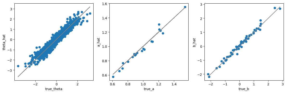
参考文献
- Masters, G. N. (1982). A Rasch Model for Partial Credit Scoring. Psychometrika, 47(2), 149–174. 10.1007/bf02296272
- Muraki, E. (1992). A GENERALIZED PARTIAL CREDIT MODEL: APPLICATION OF AN EM ALGORITHM. ETS Research Report Series, 1992(1). 10.1002/j.2333-8504.1992.tb01436.x