NGBoost

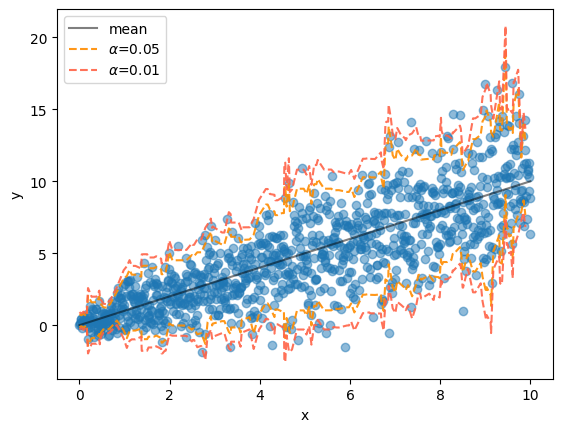
Case 1: 線形データ・不均一分散

import numpy as np
import matplotlib.pyplot as plt
from scipy.stats import norm

x = np.linspace(0, 10, 1000)
sigma = np.sqrt(x)
y = norm.rvs(loc=x, scale=sigma, random_state=0)
X = x.reshape(-1, 1)

fig, ax = plt.subplots()
ax.scatter(x, y)
ax.plot(x, x, color="black", alpha=.5, label="mean")
ax.set(xlabel="x", ylabel="y")
ax.legend()
fig.show()

from ngboost import NGBRegressor
from sklearn.model_selection import train_test_split
from sklearn.metrics import mean_squared_error

X_train, X_test, y_train, y_test = train_test_split(X, y, test_size=0.2)

ngb = NGBRegressor().fit(X_train, y_train)
y_pred = ngb.predict(X_test)
y_dist = ngb.pred_dist(X_test)

print('Test MSE', mean_squared_error(y_pred, y_test))

# test Negative Log Likelihood
test_NLL = -y_dist.logpdf(y_test).mean()
print('Test NLL', test_NLL)

[iter 0] loss=2.7024 val_loss=0.0000 scale=1.0000 norm=3.0573

[iter 100] loss=2.1664 val_loss=0.0000 scale=2.0000 norm=3.4653

[iter 200] loss=1.9810 val_loss=0.0000 scale=2.0000 norm=3.2390

[iter 300] loss=1.9152 val_loss=0.0000 scale=2.0000 norm=3.1663

[iter 400] loss=1.8766 val_loss=0.0000 scale=1.0000 norm=1.5515

Test MSE 5.800682122676115
Test NLL 2.2674320076276135

fig, ax = plt.subplots()
ax.scatter(x, y, alpha=.5)
ax.plot(x, x, color="black", alpha=.5, label="mean")
ax.set(xlabel="x", ylabel="y")
ax.legend()

X_test = np.sort(X_test, axis=0)
y_dist = ngb.pred_dist(X_test)

alphas = [0.05, 0.01]
colors = ["darkorange", "tomato"]
for alpha, color in zip(alphas, colors):
    upper = norm.ppf(q=1 - (alpha/2), loc=y_dist.params["loc"], scale=y_dist.params["scale"])
    lower = norm.ppf(q=(alpha/2), loc=y_dist.params["loc"], scale=y_dist.params["scale"])
    ax.plot(X_test[:, 0], upper, alpha=.9, color=color, linestyle="--", label=rf"$\alpha$={alpha}")
    ax.plot(X_test[:, 0], lower, alpha=.9, color=color, linestyle="--")

ax.legend()
fig.show()

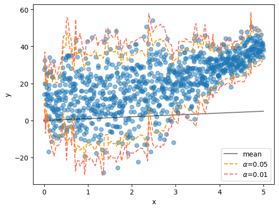
Case 2: 非線形データ・不均一分散

import numpy as np
import matplotlib.pyplot as plt
from scipy.stats import norm

x = np.linspace(0, 5, 1000)
sigma = (np.sin(x / 1) + 2) * 5
z = 10 + x + x ** 2
y = norm.rvs(loc=z, scale=sigma, random_state=0)
X = x.reshape(-1, 1)

fig, ax = plt.subplots()
ax.scatter(x, y)
ax.plot(x, z, color="black", alpha=.5, label="mean")
ax.set(xlabel="x", ylabel="y")
ax.legend()
fig.show()

from ngboost import NGBRegressor
from sklearn.model_selection import train_test_split
from sklearn.metrics import mean_squared_error

X_train, X_test, y_train, y_test = train_test_split(X, y, test_size=0.2)

ngb = NGBRegressor().fit(X_train, y_train)
y_pred = ngb.predict(X_test)
y_dist = ngb.pred_dist(X_test)

print('Test MSE', mean_squared_error(y_pred, y_test))

# test Negative Log Likelihood
test_NLL = -y_dist.logpdf(y_test).mean()
print('Test NLL', test_NLL)

[iter 0] loss=4.0867 val_loss=0.0000 scale=2.0000 norm=23.6984

[iter 100] loss=3.7024 val_loss=0.0000 scale=2.0000 norm=16.3517

[iter 200] loss=3.5836 val_loss=0.0000 scale=2.0000 norm=15.6040

[iter 300] loss=3.5348 val_loss=0.0000 scale=2.0000 norm=15.2579

[iter 400] loss=3.4939 val_loss=0.0000 scale=2.0000 norm=14.8462

Test MSE 136.5383401184266
Test NLL 3.8719614321130886

fig, ax = plt.subplots()
ax.scatter(x, y, alpha=.5)
ax.plot(x, x, color="black", alpha=.5, label="mean")
ax.set(xlabel="x", ylabel="y")
ax.legend()

X_test = np.sort(X_test, axis=0)
y_dist = ngb.pred_dist(X_test)

alphas = [0.05, 0.01]
colors = ["darkorange", "tomato"]
for alpha, color in zip(alphas, colors):
    upper = norm.ppf(q=1 - (alpha/2), loc=y_dist.params["loc"], scale=y_dist.params["scale"])
    lower = norm.ppf(q=(alpha/2), loc=y_dist.params["loc"], scale=y_dist.params["scale"])
    ax.plot(X_test[:, 0], upper, alpha=.9, color=color, linestyle="--", label=rf"$\alpha$={alpha}")
    ax.plot(X_test[:, 0], lower, alpha=.9, color=color, linestyle="--")

ax.legend()
fig.show()