連続確率分布#
正規分布#
確率変数
で与えられることをいい、この分布を
Show code cell source
import matplotlib.pyplot  as plt
from scipy.stats import norm

np.random.seed(0)
x = np.linspace(-5, 5, 100)
pdf = norm.pdf(x)

fig, ax = plt.subplots()
ax.plot(x, pdf)
ax.set(title="Normal(μ=0, σ^2=1)", xlabel="x", ylabel="probability density")
fig.show()
---------------------------------------------------------------------------
NameError                                 Traceback (most recent call last)
Cell In[1], line 4
      1 import matplotlib.pyplot  as plt
      2 from scipy.stats import norm
----> 4 np.random.seed(0)
      5 x = np.linspace(-5, 5, 100)
      6 pdf = norm.pdf(x)

NameError: name 'np' is not defined
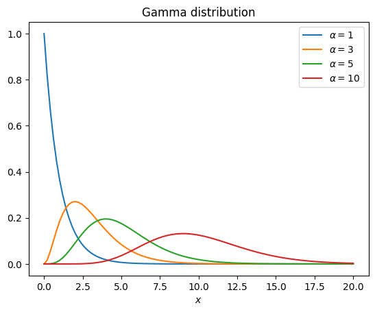
ガンマ分布#
ガンマ分布(gamma distribution)は非負の実数直線上の代表的な確率分布。その確率密度関数は
である。
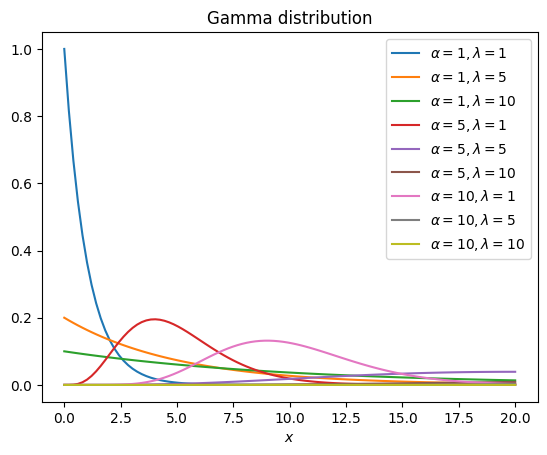
尺度変換
となる。
尺度変換
という定義も使われる(
Show code cell source
import numpy as np
import matplotlib.pyplot  as plt
from scipy.stats import gamma

x = np.linspace(0, 20, 100)

fig, ax = plt.subplots()
for alpha in [1, 3, 5, 10]:
    y = gamma.pdf(x, alpha)
    ax.plot(x, y, label=fr"$\alpha={alpha}$")
ax.legend()
ax.set(title=r"Gamma distribution", xlabel=r"$x$")
fig.show()
Show code cell source
import numpy as np
import matplotlib.pyplot  as plt
from scipy.stats import gamma

x = np.linspace(0, 20, 100)

fig, ax = plt.subplots()
for alpha in [1, 5, 10]:
    for lambda_ in [1, 5, 10]:
        y = gamma.pdf(x, alpha, scale=lambda_)
        ax.plot(x, y, label=fr"$\alpha={alpha}, \lambda={lambda_}$")
ax.legend()
ax.set(title=r"Gamma distribution", xlabel=r"$x$")
fig.show()
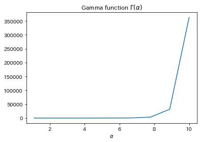
ここで
Show code cell source
from scipy.special import gamma

x = np.linspace(0, 10, 10)
y = gamma(x)

fig, ax = plt.subplots()
ax.plot(x, y)
ax.set(title=r"Gamma function $\Gamma(\alpha)$", xlabel=r"$\alpha$")
fig.show()
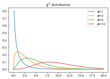
データの二乗和が従う確率分布のこと。標準正規分布に従う確率変数
カイ2乗分布の密度関数は
Show code cell source
from scipy.stats import chi2

x = np.linspace(0, 20, 100)
dfs = [1, 3, 5, 10]

fig, ax = plt.subplots()
for df in dfs:
    y = chi2.pdf(x, df=df)
    ax.plot(x, y, label=f"df={df}")
ax.legend()
ax.set(title=r"$\chi^2$ distribution")
fig.show()