区間推定#
区間推定(interval estimation)は推定したいパラメータ\(\theta\)の真の値がある区間\((L, U)\)に入る確率が\(1-\alpha\)以上(\(\alpha\)は\(\theta\)が区間に入らない確率)になる区間を推定する。つまり、
の\(L, U\)を推定する。
なお、この\(1-\alpha\)を信頼係数(confidence coefficient)といい、区間\([L, U]\)を信頼区間(confidence interval)と呼ぶ。
正規母集団の母平均の区間推定#
確率変数\(X\)の標本平均\(\bar{X}\)は中心極限定理により正規分布\(N(\mu, \sigma^2 / n)\)に従う。
これを標準化して
とすると、これは平均0、標準偏差1の標準正規分布に従う。
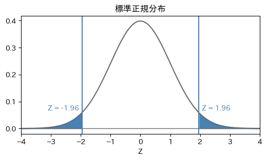
標準正規分布は\((-\infty, \infty)\)の範囲にわたって確率密度関数がゼロでない領域が存在するが、図のように正規分布の両端でそれぞれ確率\(\alpha/2\)分だけ推定を誤る可能性を許容すると、一定の範囲で区切ることができる。図は\(\alpha=0.05\)として、両側それぞれでその半分の確率\(\alpha / 2 = 0.025\)の領域で区切っており、それに相当する\(Z\)の値が\(Z \pm 1.96\)である。
一般化してこのような値を\(Z_{\alpha/2}\)と表すことにすると、区間推定は
となり、これを\(\mu\)について解くと
であり、信頼区間は
となる。
pythonでの実装#
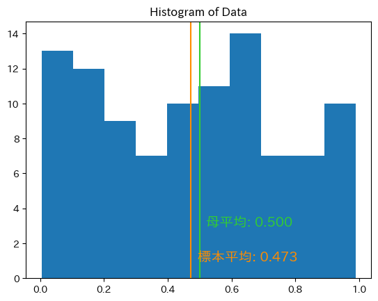
母集団が\([0, 1]\)の範囲の値をとる一様分布\(U(0, 1)\)(母平均\(\mu=\frac{0+1}{2} = 0.5\))であるとし、そこから得た次のようなサンプルがあるとする。
式をpythonに落とし込んで計算すると次のようになる
# ※ddof=1: 不偏標準偏差にするためのオプション
std_error = x.std(ddof=1) / np.sqrt(n)

# 信頼区間
alpha = 0.05
z = norm.ppf(1 - alpha / 2)
[x.mean() - z * std_error, x.mean() + z * std_error]
[0.4160030960878336, 0.5295845829372018]
statsmodelsのemplike.DescStatで計算することもできる
# statsmodelsを使う場合
from scipy.stats import norm
import statsmodels.api as sm
el = sm.emplike.DescStat(x)
el.ci_mean()
(0.4166429503391242, 0.5294769896986984)
scipy.stats の norm.interval() で計算することもできる。
from scipy.stats import norm, sem
norm.interval(confidence=0.95, loc=x.mean(), scale=sem(x))
# ※ sem は standard error of mean、つまり x.std(ddof=1) / np.sqrt(n)と等しい
(0.4160030960878336, 0.5295845829372018)
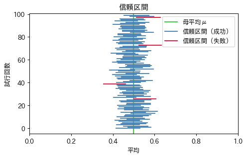
サンプルをとって95%信頼区間を計算する作業を100回繰り返したものが以下の図である。\(\alpha=0.05\)なので、100回の調査で5回程度は推定を誤る(信頼区間に母平均が含まれない)可能性がある。
\(t\)検定#
母分散が未知の場合、\(t\)分布を用いる。標本標準偏差を\(s\)とすると、
は自由度\(n-1\)の\(t\)分布に従うため、
となる。