線形回帰

線形回帰#

モデル#

線形回帰（linear regression）は、予測の目的変数 $y$ と特徴量（説明変数） $x_{1}, x_{2}, . . ., x_{d}$ の間に次のような線形関係を仮定したモデルを置いて予測する手法。 $ $y = β_{0} + β_{1} x_{1} + \dots + β_{d} x_{d} + ε$ $

ここで $β_{1}, β_{2}, . . ., β_{d}$ は回帰係数と呼ばれるパラメータで、モデル内で推定される。 $ε$ はデータ取得時の測定誤差などの偶然による誤差を表し、次の3つの条件を満たす。

期待値は0： $E [ε] = 0$
分散は一定: $V [ε] = σ^{2}$
異なった誤差項は無相関: $j \neq i$ ならば $C o v (ε_{i}, ε_{j}) = E (ε_{i}, ε_{j}) = 0$

サンプルサイズが $n$ のデータセット ${x_{i}, y_{i}}_{i = 1}^{n}$ があるとして、目的変数を $y = (y_{1}, y_{2}, . . ., y_{n})^{⊤}$ 、特徴量を $X = (x_{1}, x_{2}, . . ., x_{n})^{⊤}$ とおくと、このモデルは

y = X β + ε

と表記することができる。

パラメータの推定#

一般的に線形回帰ではパラメータの推定に最小二乗法（least squares method）という方法が使われる。

これは誤差関数 $J (β)$ を実測値 $y$ と予測値 $\hat{y} = X \hat{β}$ の二乗誤差の和（誤差二乗和 sum of squared error: SSE）

J (β) = | | y - X \hat{β} | |^{2} = \sum_{i = 1}^{n} (y_{i} - {\hat{y}}_{i})^{2} = \sum_{i = 1}^{n} ε_{i}^{2} = ε^{⊤} ε

として定義し、この二乗誤差を最小にするパラメータ（最小二乗推定量 ordinary least square’s estimator: OLSE）

{\hat{β}}^{L S} = \underset{β}{a r g m i n} \sum_{i = 1}^{n} (y_{i} - {\hat{y}}_{i})^{2}

を採用するという方法。

二乗誤差 $(y_{i} - {\hat{y}}_{i})^{2} = ε_{i}^{2}$ はU字型になるため傾きがゼロになる点が最小値になる。そのため最小二乗法は解析的に解を求めることができる。

../../../_images/edc187ce62c7bfccc48cac0aecc28ce533727b33c4d77fed6bbed4abb8838430.png

誤差二乗和は

\begin{array}{r} \begin{aligned} ε^{⊤} ε & = (y - X \hat{β})^{⊤} (y - X \hat{β}) \\ = y^{⊤} y - y^{⊤} X β - (X β)^{⊤} y + (X β)^{⊤} (X β) \\ = y^{⊤} y - 2 β^{⊤} X^{⊤} y + β^{⊤} X^{⊤} X β \end{aligned} \end{array}

であるから、二乗誤差の傾きがゼロになる点は

\frac{\partial ε^{⊤} ε}{\partial β} = - 2 X^{⊤} y + 2 (X^{⊤} X) β = 0

と表すことができる。

これを整理して

2 (X^{⊤} X) β = 2 X^{⊤} y

これの両辺を2で割ると（あるいは誤差関数の定義の際に $1 / 2$ を掛けておくと）、正規方程式（normal equation）とよばれる次の式が得られる。

(X^{⊤} X) β = X^{⊤} y

これを $β$ について解けば

β = (X^{⊤} X)^{- 1} X^{⊤} y

となり、最小二乗推定量 ${\hat{β}}^{L S}$ が得られる。

実装#

numpyでは、行列やベクトルの積は@という演算子で書くことができる。そのため、

import numpy as np
beta = np.linalg.inv(X.T @ X) @ X.T @ y

のように書けば上の式とおなじ演算を行うことができる。

データの準備#

乱数を発生させて架空のデータを作る。

\begin{array}{r} y = 10 + 3 x_{1} + 5 x_{2} + ε \\ x_{1} \sim U n i f o r m (0, 10) \\ x_{2} \sim N o r m a l (3, 1) \\ ε \sim N o r m a l (0, 1) \end{array}

ここで $ε$ は測定誤差などのランダムなノイズとする

import numpy as np
import pandas as pd
n = 100  # sample size

np.random.seed(0)
x0 = np.ones(shape=(n, ))
x1 = np.random.uniform(0, 10, size=n)
x2 = np.random.normal(3, 1, size=n)
noise = np.random.normal(size=n)

beta = [10, 3, 5]  # 真の回帰係数
y = beta[0] * x0 + beta[1] * x1 + beta[2] * x2 + noise 

特徴量 $x$ と目的変数 $y$ の関係を散布図で描くと次の図のようになった。

[Text(0.5, 0, 'x2'), Text(0, 0.5, 'y')]

../../../_images/601679470e8940cbec02cb5fa0cac7c0e1acd14cfcd95805ab10cc18f1d0facb.png

推定#

これらのデータを使用して推定を行う。

X = np.array([x0, x1, x2]).T

# Xの冒頭5行は以下のようになっている
print(X[0:5])

[[1.         5.48813504 1.83485016]
 [1.         7.15189366 3.90082649]
 [1.         6.02763376 3.46566244]
 [1.         5.44883183 1.46375631]
 [1.         4.23654799 4.48825219]]

# 最小二乗法で推定
beta_ = np.linalg.inv(X.T @ X) @ X.T @ y

print(f"""
推定された回帰係数: {beta_.round(3)}
データ生成過程の係数: {beta}
""")

推定された回帰係数: [9.564 2.98  5.119]
データ生成過程の係数: [10, 3, 5]

真の値にそれなりに近い回帰係数が推定できた。

なお、scikit-learnに準拠したfit/predictのメソッドを持つ形でクラスとして定義するなら、以下のようになる（参考： sklearn準拠モデルの作り方 - Qiita）。

# scikit-learnに準拠した形で実装
from sklearn.base import BaseEstimator, RegressorMixin


class LinearRegression(BaseEstimator, RegressorMixin):

    def fit(self, X, y):
        self.coef_ = np.linalg.inv(X.T @ X) @ X.T @ y
        return self

    def predict(self, X):
        return X @ self.coef_

model = LinearRegression()
model.fit(X, y)
model.coef_

array([9.56372548, 2.97972446, 5.11931302])

予測してみる#

root mean squared error (RMSE)

R M S E = \sqrt{\frac{1}{N} \sum_{i = 1}^{N} (y_{i} - {\hat{y}}_{i})^{2}}

を使って予測値を評価してみる。

# 予測値を算出
y_pred = model.predict(X)

# 予測誤差を評価
from sklearn.metrics import mean_squared_error
rmse = mean_squared_error(y, y_pred, squared=False)

print(f"RMSE: {rmse:.3f}")

---------------------------------------------------------------------------
TypeError                                 Traceback (most recent call last)
Cell In[8], line 6
      4 # 予測誤差を評価
      5 from sklearn.metrics import mean_squared_error
----> 6 rmse = mean_squared_error(y, y_pred, squared=False)
      8 print(f"RMSE: {rmse:.3f}")

File /usr/local/lib/python3.10/site-packages/sklearn/utils/_param_validation.py:194, in validate_params.<locals>.decorator.<locals>.wrapper(*args, **kwargs)
    191 func_sig = signature(func)
    193 # Map *args/**kwargs to the function signature
--> 194 params = func_sig.bind(*args, **kwargs)
    195 params.apply_defaults()
    197 # ignore self/cls and positional/keyword markers

File /usr/local/lib/python3.10/inspect.py:3186, in Signature.bind(self, *args, **kwargs)
   3181 def bind(self, /, *args, **kwargs):
   3182     """Get a BoundArguments object, that maps the passed `args`
   3183     and `kwargs` to the function's signature.  Raises `TypeError`
   3184     if the passed arguments can not be bound.
   3185     """
-> 3186     return self._bind(args, kwargs)

File /usr/local/lib/python3.10/inspect.py:3175, in Signature._bind(self, args, kwargs, partial)
   3173         arguments[kwargs_param.name] = kwargs
   3174     else:
-> 3175         raise TypeError(
   3176             'got an unexpected keyword argument {arg!r}'.format(
   3177                 arg=next(iter(kwargs))))
   3179 return self._bound_arguments_cls(self, arguments)

TypeError: got an unexpected keyword argument 'squared'

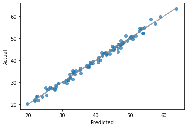
予測値と実測値の散布図を描くと次のようになった。

[Text(0.5, 0, 'Predicted'), Text(0, 0.5, 'Actual')]

../../../_images/0076c3a74b0c4c769a504419d2c3f557039d257d9e833a6cf897e349436d2a60.png