分位点回帰

分位点\(\tau\)における条件付分位関数を

\[ Q_\tau(y_i | X_i) = F_y^{-1}(\tau | X_i) \]

と表す。ここで\(F_y^{-1}(\tau | X_i)\)は\(y\)において\(X_i\)に条件づけられた\(y_i\)の分布関数である（\(F_y^{-1}(\tau | X_i) = \inf \{ y: F_y(y|X_i) \geq \tau \}\)）。

例えば\(\tau = 0.1\)のとき、\(Q_\tau(y_i | X_i)\)は\(y_i\)の下位10分位である。

標準的な回帰モデルは二乗誤差\((y_i - m(X_i))^2\)の和や期待値を最小化するようにモデル\(m(X_i)\)を学習して条件付き期待値\(E(y_i|X_i)\)を予測する

\[ \newcommand{\argmin}{\mathop{\rm arg~min}\limits} E(y_i|X_i) = \argmin_{m(X_i)} E\big[ (y_i - m(X_i))^2 \big] \]

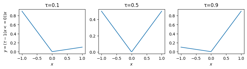
分位点回帰 （quantile regression）モデルはpinball loss\(\rho_{\tau}(y_i - q(X_i))\)の和や期待値を最小化するようにモデル\(q(X_i)\)を学習させ、条件付き分位関数\(Q_{\tau}(y_i|X_i) = F^{-1}_y(\tau|X_i)\)を予測する

\[ Q_{\tau}(y_i|X_i) = \argmin_{q(X_i)} E\big[ \rho_{\tau}(y_i - q(X_i)) \big] \]

pinball lossは \(\tau\)-tiled absolute value function や 検定関数（check function）とも呼ばれる（グラフを描くとチェックマークに似てるため）

\[ \rho_{\tau} (x) = \big(\tau - \mathbb{1}(x \leq 0) \big) x \]

あるいは

\[\begin{split} \rho_{\tau} (x) = \begin{cases} (\tau - 1) x & \text{ if } x \leq 0\\ \tau x & \text{ if } x > 0\\ \end{cases} \end{split}\]

と書かれる

\[ \rho_{\tau} (x) = \big(\tau - \mathbb{1}(x \leq 0) \big) x \]

は

\(x \leq 0\)のときは

\[ \big(\tau - \mathbb{1}(x \leq 0) \big) x = (\tau - 1) x \]

となり、

\(x > 0\)のときは

\[ \big(\tau - \mathbb{1}(x \leq 0) \big) x = (\tau - 0) x = \tau x \]

となるので、

\[\begin{split} \rho_{\tau} (x) = \begin{cases} (\tau - 1) x & \text{ if } x \leq 0\\ \tau x & \text{ if } x > 0\\ \end{cases} \\ = \big(\tau - \mathbb{1}(x \leq 0) \big) x \end{split}\]

Show code cell source Hide code cell source

import numpy as np
import matplotlib.pyplot as plt

def pinball_loss(x, tau):
    return (tau - 1 * (x <= 0)) * x

x = np.linspace(-1, 1, 100)
fig, axes = plt.subplots(figsize=[10, 2], ncols=3)
for i, tau in enumerate([0.1, 0.5, 0.9]):
    y = pinball_loss(x, tau=tau)
    axes[i].plot(x, y)
    if i == 0:
        axes[i].set(title=f"τ={tau}", xlabel=r"$x$", ylabel=r"$y = (\tau - 1(x <= 0)) x$")
    else:
        axes[i].set(title=f"τ={tau}", xlabel=r"$x$")
fig.show()

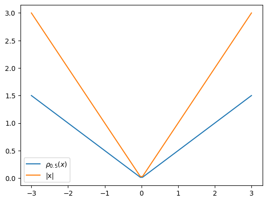
なお、pinball lossは\(\tau=0.5\)のとき

\[\begin{split} \begin{align} \rho_{0.5} (x) &= \begin{cases} -0.5 x & \text{ if } x \leq 0\\ 0.5 x & \text{ if } x > 0\\ \end{cases} \\ &= \frac{1}{2} |x| \end{align} \end{split}\]

と、絶対誤差と比例する形になる。

絶対誤差の和を目的関数にとった線形モデルは統計学においてleast absolute deviations (LAD) と呼ばれ、その解は条件付き中央値になる

\[ \text{median}(y_i|X_i) = Q_{0.5}(y_i|X_i) = \argmin_{q(X_i)} E\big[ \rho_{0.5}(y_i - q(X_i)) \big] \]

Show code cell source Hide code cell source

import numpy as np
import matplotlib.pyplot as plt

def pinball_loss(x, tau):
    return (tau - 1 * (x <= 0)) * x

x = np.linspace(-3, 3, 100)
fig, ax = plt.subplots()
ax.plot(x, pinball_loss(x, tau=0.5), label=r"$\rho_{0.5}(x)$")
ax.plot(x, abs(x), label="|x|")
ax.legend()
fig.show()

モデルの評価

D2 pinball score

\(D^2\)は\(R^2\)の一般化

\[ D^2(y, \hat{y}) = 1 - \frac{\text{dev}(y, \hat{y})}{\text{dev}(y, y_{\text{null}})} \]

ここで\(y_{\text{null}}\)は切片のみのモデルの最適解（例：二乗誤差なら\(y\)の平均値、絶対誤差なら\(y\)の中央値、pinball lossなら\(y\)の指定されたquantile）

この\(D^2\)に

\[ \text{dev}(y, \hat{y}) = \text{pinball}(y, \hat{y}) \]

を代入したものが\(D^2\) pinball score

interval score

• [2011.09588] Beyond Pinball Loss: Quantile Methods for Calibrated Uncertainty Quantification

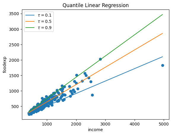
分位点回帰モデルの実践

statsmodelsでは quantreg() で実行できる

Quantile regression - statsmodels 0.15.0 (+213)

Show code cell source Hide code cell source

import numpy as np
import pandas as pd
import statsmodels.api as sm
import statsmodels.formula.api as smf
import matplotlib.pyplot as plt

data = sm.datasets.engel.load_pandas().data

fig, ax = plt.subplots()
ax.scatter(data["income"], data["foodexp"])
ax.set(xlabel="income", ylabel="foodexp", title="Quantile Linear Regression")

x = np.linspace(data["income"].min(), data["income"].max(), 10)
model = smf.quantreg("foodexp ~ income", data)
for q in [0.1, 0.5, 0.9]:
    res = model.fit(q=q)
    y_hat = res.predict(pd.DataFrame({"income": x}))
    ax.plot(x, y_hat, label=fr"$\tau = {q}$")
ax.legend()
fig.show()