MIC(Maximal Information Coefficient)#
Reshef, et al. (2011). Detecting novel associations in large data sets. で提案されたMIC(Maximal Information Coefficient)は、相互情報量を用いてデータの非線形な関連性を評価できる係数。
「21世紀の相関係数(A Correlation for the 21st Century)」としてScience誌に紹介され、話題になった。
相互情報量(Mutual Information; MI)#
確率分布 \(p(x,y)\) による一般の非線形依存関係の強さを測る。
定義式#
離散確率変数の場合:
\[
I(X ; Y)=\sum_{y \in \mathcal{Y}} \sum_{x \in \mathcal{X}} p(x, y) \log \frac{p(x, y)}{p(x) p(y)}
\]
連続確率変数の場合:
\[
I(X ; Y)=\int_{\mathcal{Y}} \int_{\mathcal{X}} p(x, y) \log \frac{p(x, y)}{p(x) p(y)} d x d y
\]
特徴#
\(I(X;Y)=0\) なら 独立
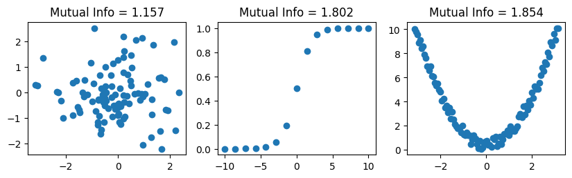
線形・非線形を問わずあらゆる依存を検出
ただし値域が固定されておらず、相関係数のように簡単には解釈できない
推定には KDE, kNN などが必要
MIC(Maximal Information Coefficient)#
概念的な定義#
散布図をさまざまな格子分割 \((x,y)\) に切り、各ビンの相対頻度から 相互情報量 を計算し、その最大値をスケール正規化したもの。
MIC は相互情報量を複数グリッドで最大化し、
\[
0 \le \mathrm{MIC} \le 1
\]
となるように正規化した指標。
特徴#
単調・非単調のどちらも検出
関係の形状が分からない探索フェーズに強い
計算はやや重いが実務では十分使える