ベクトル自己回帰(VAR)モデル#
VARはARモデルの拡張版であり、VAR(\(p\))モデルは\(y_t\)を定数と自身の\(p\)次のラグ(\(p\)期の過去の値)に回帰したモデル。
モデル#
変数が\(n\)次元、ラグの次数が\(p\)だとする。(例えば時点\(t\)の観測値は \(y_{1,t}, y_{2,t}, \dots, y_{n,t}\) となる。)
VAR(\(p\)) では、各変数 \(y_{i,t}\) は、すべての変数の過去 \(p\) 期分の線形結合で表される。
\(\phi_{ij}^{(k)}\):変数 \(j\) の \(k\) 期前」が「変数 \(i\) の現在」に与える影響
\(\varepsilon_{i,t}\):変数 \(i\) に対応する誤差項
もう少しベクトルや行列を使って表すと、
\(\mathbf{c}\in\mathbb{R}^{n\times 1}\)
\(\boldsymbol{\Phi}_k \in\mathbb{R}^{n\times n}\)
ここで \(\rho=\operatorname{Corr}\left(\varepsilon_{1 t}, \varepsilon_{2 t}\right)\)
状態ベクトル \(\mathbf{y}_t \in \mathbb{R}^n\) 、 ラグ \(k\) の係数行列 \(\boldsymbol{Phi}_k \in \mathbb{R}^{n \times n}\)、 誤差ベクトル \(\boldsymbol{\varepsilon}_t\) をそれぞれ
とおくと、VAR(\(p\)) は次のように表現できる。
※切片を含めた表現もされる
パラメータ推定#
VARは一見複雑だが、本質的には各変数を同じ説明変数で回帰しているだけ(多変量回帰)である。例えばVAR(1) は \(\mathbf{y}_t = \mathbf{\Phi}_1 \mathbf{y}_{t-1} + \boldsymbol{\varepsilon}_t\) 。
サンプルサイズを \(T\) とする(初期 \(p\) 個は捨てる)。
目的変数行列を\(\mathbf{Y}\)、説明変数行列を\(\mathbf{Z}\)、係数行列をまとめたものを\(\mathbf{B}\)とおく。
VARはOLSで推定可能
実装#
Vector Autoregressions tsa.vector_ar - statsmodels 0.14.6
import numpy as np
import pandas
import statsmodels.api as sm
from statsmodels.tsa.api import VAR

mdata = sm.datasets.macrodata.load_pandas().data

# prepare the dates index
dates = mdata[['year', 'quarter']].astype(int).astype(str)
quarterly = dates["year"] + "Q" + dates["quarter"]

from statsmodels.tsa.base.datetools import dates_from_str
quarterly = dates_from_str(quarterly)

mdata = mdata[['realgdp', 'realcons']]
mdata.index = pandas.DatetimeIndex(quarterly)
data = np.log(mdata).diff().dropna()

# data
display(data.tail())

# make a VAR model
model = VAR(data)
results = model.fit(2)
results.summary()
| realgdp | realcons | |
|---|---|---|
| 2008-09-30 | -0.006781 | -0.008948 |
| 2008-12-31 | -0.013805 | -0.007843 |
| 2009-03-31 | -0.016612 | 0.001511 |
| 2009-06-30 | -0.001851 | -0.002196 |
| 2009-09-30 | 0.006862 | 0.007265 |
/home/runner/work/notes/notes/.venv/lib/python3.10/site-packages/statsmodels/tsa/base/tsa_model.py:473: ValueWarning: No frequency information was provided, so inferred frequency QE-DEC will be used.
  self._init_dates(dates, freq)
  Summary of Regression Results
==================================
Model:                         VAR
Method:                        OLS
Date:           Sun, 21, Jun, 2026
Time:                     23:33:23
--------------------------------------------------------------------
No. of Equations:         2.00000    BIC:                   -20.0648
Nobs:                     200.000    HQIC:                  -20.1630
Log likelihood:           1465.40    FPE:                1.63813e-09
AIC:                     -20.2297    Det(Omega_mle):     1.55920e-09
--------------------------------------------------------------------
Results for equation realgdp
==============================================================================
                 coefficient       std. error           t-stat            prob
------------------------------------------------------------------------------
const               0.001024         0.000971            1.055           0.291
L1.realgdp         -0.096477         0.087307           -1.105           0.269
L1.realcons         0.571453         0.102953            5.551           0.000
L2.realgdp         -0.038461         0.081226           -0.474           0.636
L2.realcons         0.352325         0.109914            3.205           0.001
==============================================================================

Results for equation realcons
==============================================================================
                 coefficient       std. error           t-stat            prob
------------------------------------------------------------------------------
const               0.004668         0.000843            5.538           0.000
L1.realgdp          0.051847         0.075826            0.684           0.494
L1.realcons         0.194414         0.089414            2.174           0.030
L2.realgdp          0.013699         0.070545            0.194           0.846
L2.realcons         0.181398         0.095460            1.900           0.057
==============================================================================

Correlation matrix of residuals
             realgdp  realcons
realgdp     1.000000  0.603188
realcons    0.603188  1.000000
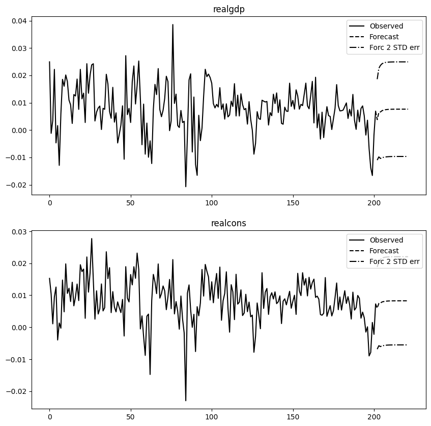
_ = results.plot_forecast(steps=20)