一般化部分採点モデル#
概要#
一般化部分得点モデル(Generalized Partial Credit Model: GPCM, Muraki, 1992) は多値の順序尺度の反応を扱えるIRTモデル。
一般化部分得点モデル(Generalized Partial Credit Model: GPCM)
被験者 \(i\)、項目 \(j\)、カテゴリ \(k = 1,\dots,K\) に対して
\(a_j\):項目 \(j\) の識別力
\(b_{jk}\):段階 \(k-1 \to k\) の困難度
GRMとGPCMの使い分けについて#
SATの実世界データとシミュレーションデータを使ってGPCMとGRMを比較した。
\(\theta\)の推定値は相関係数 0.9748 ~ 0.9921と高い相関を示した。
データ:Rの
irtplayパッケージのsimdat()関数で、GRMとGPCMの下でのデータを生成。異なるサンプルサイズ・項目数・欠損率で比較。GRM生成データをGPCMで分析すると収束しないケースが多い→やはり両モデルは若干異なる
項目母数の安定性:GPCM > GRM
能力母数の精度:GRM > GPCM(ただし高欠測率の時はGPCMが安定)
テスト情報量はGRMが高くなる傾向がある
考え方#
隣のカテゴリとの2択で考える#
2カテゴリの場合#
\(y_{ij}\in\{0,1\}\)とする。2PLモデルにおいては、
「\(y_{ij}=0\)の確率(カテゴリ0を選ぶ確率)」と「\(y_{ij}=1\)の確率(カテゴリ1を選ぶ確率)」の合計は1になる。そして「カテゴリ1を選ぶ確率」は
と表すことができる。
\(K\)カテゴリの場合#
これを\(K\)カテゴリ(\(k=1,2,\cdots,K\))に一般化し、「隣り合う2つのカテゴリ\(k-1\)と\(k\)の二択において\(k\)を選ぶ確率」\(P(y_{i j}^*=k)_{k-1, k}\)とする。
これは反応 \(y_{ij}\) が \(k-1\) か \(k\) のどちらかだと仮定して正規化したとき、\(k\) が選ばれる「相対的な割合」。
式\((1)\)を
\(P(y_{ij}=k)=\)の形に変形すると
となる。
式変形メモ
わかりやすくするため、記号を単純化する。
まず
の両辺に \(P_k+P_{k-1}\) を掛ける:
左辺を展開:
\(P_k\) を左にまとめる:
両辺を \(1-P^*\) で割る:
漸化式の形に変形#
ここで、\(k\)と\(k-1\)のカテゴリの2択であるということで、2PLMと同様にロジスティックモデルで表現できるとすると、
と対数オッズを線形モデルで表現する形に表すことができる。この両辺に指数をとると
になる。簡単のため\(\pi_{ijk} = a_j(\theta_i-b_{j k})\)とすると、式\((2)\)は
という漸化式の形になる。言葉で書くと、「特定のカテゴリ\(k\)を選ぶ確率 \(P(y_{ij}=k)\) 」は、「 \(k-1\) を選ぶ確率 \(P(y_{ij}=k-1)\) 」と「隣のカテゴリに移るオッズ\(\exp(\pi_{ijk}) = \frac{P(y_{i j}^*=k)_{k-1, k}}{1-P(y_{i j}^*=k)_{k-1, k}}\) 」で表すことができるというもの。
例えば3カテゴリの場合は
のようになる。つまり、\(P(y_{ij}=1)\)に\(\exp(\pi_{ijk})\)の積を掛け合わせた形ですべてのカテゴリの反応確率が表される。
いったん\(\pi_{ij1} = 0\)として、\(P(y_{ij}=1) = \exp(\pi_{ij1}) = 1\) を代入すると
正規化#
\(P(y_{ij}=1)=1\)としたため、全カテゴリの選択確率の総和が1になるとは限らない。そこで全カテゴリの総和で割って正規化する。
項目特性曲線#
項目特性曲線(ICC)あるいは CRC(Category Response Curves) は 能力 \(\theta\) に対して各カテゴリ \(k\) が選ばれる確率 \(P(Y=k\mid\theta)\) を描いた曲線群
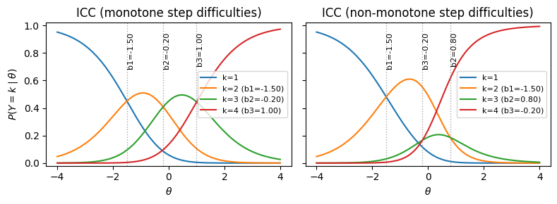
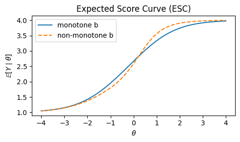
また、全体の傾向を見たい場合は能力 \(\theta\) におけるその項目の期待得点(得点で重みづけたCRC)である ESC(Expected Score Curve)
というものがある。
# ESC(単調ケース)
E_mono = np.sum((np.arange(1, K+1)[None, :]) * P_mono, axis=1)

# ESC(非単調ケース)
E_nonmono = np.sum((np.arange(1, K+1)[None, :]) * P_nonmono, axis=1)

plt.figure(figsize=(5, 3))
plt.plot(theta, E_mono, label="monotone b")
plt.plot(theta, E_nonmono, linestyle="--", label="non-monotone b")

plt.xlabel(r"$\theta$")
plt.ylabel(r"$\mathbb{E}[Y\mid\theta]$")
plt.title("Expected Score Curve (ESC)")
plt.legend()
plt.tight_layout()
plt.show()
部分得点モデル#
部分得点モデル(Partial Credit Model: PCM, Masters, 1982) は Raschモデルを順序多値に拡張した IRT モデル。
あるいはロジットで表すと
PCMでは識別力パラメータは 存在しない(全部共通で\(a=1\))ため扱いにくく、一般化したGPCMが提案された
一般化部分得点モデル#
一般化部分得点モデル(Generalized Partial Credit Model: GPCM, Muraki, 1992) はPCMを一般化し、項目ごとに異なる識別力\(a_j\)を導入したモデル。
あるいは
\(a_j > 0\):項目 \(j\) の識別力
\(b_{jk}\):段階 \(k-1 \to k\) の難易度
実装#
最尤推定ならRのmirtパッケージでgpcmを選ぶだけだが、ベイズモデリングはややこしい
BUGS#
1	model {
2	    for (i in 1:n) {
3	        for (j in 1:p) {
4	                Y[i, j] ~ dcat(prob[i, j, 1:K[j]])
5	                }
6	                theta[i] ~ dnorm(mu0, tau0)
7	    }
8	    for (i in 1:n) {
9	        for (j in 1:p) {
10	            for (k in 1:K[j] ) {
11	                eta[i, j, k] <- alpha[j] * (theta[i] - beta[j, k])
12	                psum[i, j, k] <- sum(eta[i, j, 1:k])
13	                exp.psum[i, j, k] <- exp(psum[i, j, k])
14	                prob[i, j, k] <- exp.psum[i, j, k] / sum(exp.psum[i, j, 1:K[j]])
15	    } } }
16	    for (j in 1:p) {
17	        alpha[j] ~ dlnorm(m.alpha, pr.alpha)
18	        beta[j, 1] <- 0.0
19	        for (k in 2:K[j]) {
20	                beta[j, k] ~ dnorm(m.beta, pr.beta)
21	        }
22	    }
23	    pr.alpha <- pow(s.alpha, −2)
24	    pr.beta <- pow(s.beta, −2)
25	mu0 ~ dnorm(0, 0.01)
26	tau0 ~ dgamma(0.5, 0.5)
27	var0 <- 1/tau0
28	}
PyMC#
# データを生成
import numpy as np
import pandas as pd

def simulate_gpcm(N=1000, J=10, K=4, seed=42):
    rng = np.random.default_rng(seed)
    theta = rng.normal(0, 1, size=N)
    a = rng.lognormal(0, 0.3, size=J)
    b = rng.normal(0, 1, size=(J, K - 1))  # step difficulties(順序制約なし)

    U = np.zeros((N, J), dtype=int)
    for j in range(J):
        inc = a[j] * (theta[:, None] - b[j][None, :])  # (N, K-1)
        csum = np.cumsum(inc, axis=1)                    # (N, K-1)
        log_num = np.concatenate([np.zeros((N, 1)), csum], axis=1)  # (N, K)
        mx = log_num.max(axis=1, keepdims=True)
        exp_shift = np.exp(log_num - mx)
        P = exp_shift / exp_shift.sum(axis=1, keepdims=True)
        for i in range(N):
            U[i, j] = rng.choice(K, p=P[i])
    return U, theta, a, b

num_users = 1000
num_items = 20
U, true_theta, true_a, true_b = simulate_gpcm(N=num_users, J=num_items)
df = pd.DataFrame(
    U,
    index=[f"user_{i+1}" for i in range(num_users)],
    columns=[f"question_{j+1}" for j in range(num_items)],
)

# 縦持ちへ変換
user_categories = [f"user_{i+1}" for i in range(num_users)]
item_categories = [f"question_{j+1}" for j in range(num_items)]

df_long = pd.melt(
    df.reset_index(), id_vars="index", var_name="item", value_name="response",
).rename(columns={"index": "user"})
df_long["user"] = pd.Categorical(df_long["user"], categories=user_categories, ordered=True)
df_long["item"] = pd.Categorical(df_long["item"], categories=item_categories, ordered=True)

df_long.head()
| user | item | response | |
|---|---|---|---|
| 0 | user_1 | question_1 | 0 |
| 1 | user_2 | question_1 | 0 |
| 2 | user_3 | question_1 | 3 |
| 3 | user_4 | question_1 | 2 |
| 4 | user_5 | question_1 | 0 |
import pymc as pm
import pytensor.tensor as pt

user_idx = df_long["user"].cat.codes.to_numpy()
users = df_long["user"].cat.categories.to_numpy()
item_idx = df_long["item"].cat.codes.to_numpy()
items = df_long["item"].cat.categories.to_numpy()
responses = df_long["response"].to_numpy().astype("int64")

K = int(responses.max() + 1)
n_steps = K - 1

coords = {
    "user": users,
    "item": items,
    "step": np.arange(n_steps),
    "obs_id": np.arange(len(df_long)),
}

with pm.Model(coords=coords) as model:
    user_idx_ = pm.Data("user_idx", user_idx, dims="obs_id")
    item_idx_ = pm.Data("item_idx", item_idx, dims="obs_id")
    responses_ = pm.Data("responses", responses, dims="obs_id")

    theta = pm.Normal("theta", 0, 1, dims="user")
    a = pm.LogNormal("a", 0, 0.5, dims="item")
    b = pm.Normal("b", 0, 2, dims=("item", "step"))

    # GPCM: logit_k = sum_{c=0}^{k-1} a_j (theta_i - b_{jc}),  logit_0 = 0
    inc = a[item_idx_][:, None] * (theta[user_idx_][:, None] - b[item_idx_])
    csum = pt.cumsum(inc, axis=1)
    logits = pt.concatenate([pt.zeros_like(csum[:, :1]), csum], axis=1)

    p = pt.special.softmax(logits, axis=-1)
    pm.Categorical("obs", p=p, observed=responses_, dims="obs_id")
%%time
with model:
    idata = pm.sample(random_seed=0, draws=1000)
Initializing NUTS using jitter+adapt_diag...
Multiprocess sampling (2 chains in 2 jobs)
NUTS: [theta, a, b]
---------------------------------------------------------------------------
ValueError                                Traceback (most recent call last)
File <timed exec>:2

File ~/work/notes/notes/.venv/lib/python3.10/site-packages/pymc/sampling/mcmc.py:957, in sample(draws, tune, chains, cores, random_seed, progressbar, progressbar_theme, step, var_names, nuts_sampler, initvals, init, jitter_max_retries, n_init, trace, discard_tuned_samples, compute_convergence_checks, keep_warning_stat, return_inferencedata, idata_kwargs, nuts_sampler_kwargs, callback, mp_ctx, blas_cores, model, compile_kwargs, **kwargs)
    953 t_sampling = time.time() - t_start
    955 # Packaging, validating and returning the result was extracted
    956 # into a function to make it easier to test and refactor.
--> 957 return _sample_return(
    958     run=run,
    959     traces=trace if isinstance(trace, ZarrTrace) else traces,
    960     tune=tune,
    961     t_sampling=t_sampling,
    962     discard_tuned_samples=discard_tuned_samples,
    963     compute_convergence_checks=compute_convergence_checks,
    964     return_inferencedata=return_inferencedata,
    965     keep_warning_stat=keep_warning_stat,
    966     idata_kwargs=idata_kwargs or {},
    967     model=model,
    968 )

File ~/work/notes/notes/.venv/lib/python3.10/site-packages/pymc/sampling/mcmc.py:1042, in _sample_return(run, traces, tune, t_sampling, discard_tuned_samples, compute_convergence_checks, return_inferencedata, keep_warning_stat, idata_kwargs, model)
   1040 # Pick and slice chains to keep the maximum number of samples
   1041 if discard_tuned_samples:
-> 1042     traces, length = _choose_chains(traces, tune)
   1043 else:
   1044     traces, length = _choose_chains(traces, 0)

File ~/work/notes/notes/.venv/lib/python3.10/site-packages/pymc/backends/base.py:624, in _choose_chains(traces, tune)
    622 lengths = [max(0, len(trace) - tune) for trace in traces]
    623 if not sum(lengths):
--> 624     raise ValueError("Not enough samples to build a trace.")
    626 idxs = np.argsort(lengths)
    627 l_sort = np.array(lengths)[idxs]

ValueError: Not enough samples to build a trace.
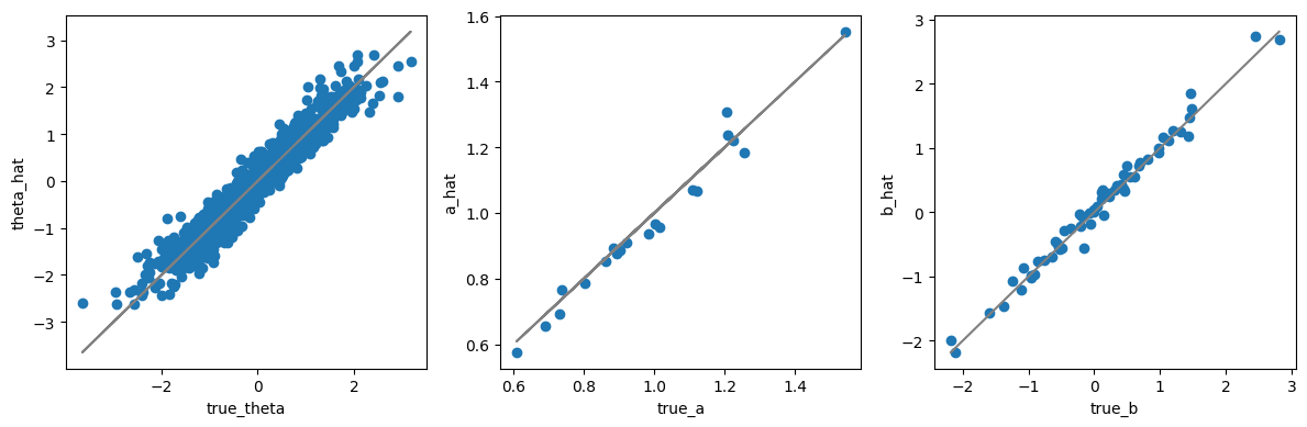
import matplotlib.pyplot as plt

post_mean = idata.posterior.mean(dim=["chain", "draw"])

fig, axes = plt.subplots(figsize=[12, 4], ncols=3)

ax = axes[0]
ax.scatter(true_theta, post_mean["theta"])
ax.plot(true_theta, true_theta, color="gray")
_ = ax.set(xlabel="true_theta", ylabel="theta_hat")

ax = axes[1]
ax.scatter(true_a, post_mean["a"])
ax.plot(true_a, true_a, color="gray")
_ = ax.set(xlabel="true_a", ylabel="a_hat")

ax = axes[2]
b_true = true_b.flatten()
b_hat = post_mean["b"].to_numpy().flatten()
ax.scatter(b_true, b_hat)
lims = [b_true.min(), b_true.max()]
ax.plot(lims, lims, color="gray")
_ = ax.set(xlabel="true_b", ylabel="b_hat")

plt.tight_layout()