一般化加法モデル (GAM)#
概要#
一般化加法モデル(Generalized Additive Models, GAM) は、Hastie と Tibshirani が 1986 年の論文
Hastie, T., & Tibshirani, R. (1986). Generalized additive models. Statistical Science, 1(3), 297–310.
で提案した統計モデル。
一般化線形モデル(GLM)は応答変数の平均 \(\mu\) と線形予測子 \(\eta = \mathbf{x}^\top \boldsymbol{\beta}\) をリンク関数 \(g\) で結ぶ。しかし線形予測子は各特徴量の効果が 線形 であると仮定しており、非線形な関係を柔軟に表現できない。
GAM は線形予測子を 滑らかな非線形関数の和(加法的構造) に置き換えることで、解釈可能性を保ちながら非線形性を扱う。
各説明変数の効果を個別に可視化できる(部分依存プロットが自然に得られる)
非線形効果を柔軟にモデリングできる
ブラックボックスな機械学習手法とは異なり、各変数の貢献が明示的
→ 交互作用項を入れたGA\(^2\)M、Explainable Boosting Machineといった説明性の高い機械学習手法へ発展していった
Hastie & Tibshirani (1986) の論文は GAM の枠組みを整備し、バックフィッティング(backfitting)アルゴリズムという実用的な推定法を提案した点で重要である。
モデル#
加法モデル#
応答変数 \(Y\) と説明変数 \(X_1, \dots, X_p\) について、加法モデル(additive model)は
と表される。ここで
\(\alpha\) は切片
\(f_j : \mathbb{R} \to \mathbb{R}\) は各説明変数に対する 非線形の滑らかな関数(スムーザー)
\(\varepsilon\) は平均ゼロの誤差項
である。識別可能性(identifiability)のため、各 \(f_j\) には \(\mathbb{E}[f_j(X_j)] = 0\) という中心化の制約を課す。
線形モデルは \(f_j(X_j) = \beta_j X_j\) の特殊ケースである。
一般化加法モデル#
Hastie & Tibshirani (1986) はこれを GLM の枠組みへ拡張した。応答変数の条件付き平均 \(\mu = \mathbb{E}[Y \mid X_1, \dots, X_p]\) に対して、リンク関数 \(g\) を用いて
とモデル化する。
応答変数の分布 |
リンク関数 \(g\) |
モデル |
|---|---|---|
正規分布 |
\(g(\mu) = \mu\)(恒等写像) |
加法モデル |
ベルヌーイ分布 |
\(g(\mu) = \log\frac{\mu}{1-\mu}\)(ロジット) |
加法ロジスティック回帰 |
ポアソン分布 |
\(g(\mu) = \log(\mu)\)(対数) |
加法ポアソン回帰 |
滑らか関数 \(f_j\) の表現#
滑らか関数 \(f_j\) の具体的な形は事前に固定せず、データから推定する。代表的な選択肢は:
スプライン(cubic spline): 結節点(knot)を設けた区分多項式
LOESS / 局所多項式回帰: 局所加重回帰(→ LOWESSのノート も参照)
カーネル回帰: 重み関数を用いた局所平均
自然スプライン(natural spline)
各 \(f_j\) の滑らかさは、平滑化パラメータ(スパン、バンド幅、自由度)で制御する。
アルゴリズム:バックフィッティング#
問題設定#
\(n\) 個のサンプル \((\mathbf{x}_i, y_i)\)、\(i = 1, \dots, n\) において、\(\mathbf{x}_i = (x_{i1}, \dots, x_{ip})\) とする。
加法モデルの目的関数(正規誤差の場合)は
第2項は \(f_j\) の曲率に対するペナルティで、\(\lambda_j \geq 0\) は滑らかさを制御するパラメータである。
バックフィッティングアルゴリズム#
Hastie & Tibshirani (1986) が提案したバックフィッティングは、各 \(f_j\) を交互に更新する座標降下法的アプローチである。
アイデア: \(j\) 番目の関数 \(f_j\) を推定する際、他の関数の寄与を除いた 部分残差(partial residual) に対してスムーザーを適用する。
backfitting
初期化:
繰り返し (収束まで):
ここで \(\mathcal{S}_j[\cdot]\) は \(j\) 番目の変数に対するスムーザーである。すなわち、入力 \(\{x_{ij}\}\) と目標値 \(\{r_{ij}\}\)(部分残差)のペアに対してスムージングを行い、各点での推定値 \(\hat{f}_j(x_{ij})\) を返す写像である。
収束#
Buja, Hastie & Tibshirani (1989) により、スムーザーが線形かつ対称半正定値である(例:スプラインスムーザー)場合、バックフィッティングは一意な解に収束することが示されている。
収束の判定は、前のイテレーションからの関数の変化量
が十分小さくなったときに行う。
GAM における IRLS との組み合わせ#
非正規分布(ロジスティック、ポアソンなど)の場合、GLM の 反復再重み付き最小二乗法(IRLS: Iteratively Reweighted Least Squares) とバックフィッティングを組み合わせる。
具体的には、各 IRLS ステップで調整済み応答変数(adjusted dependent variable)
を計算し、これに対して重み \(w_i = 1 / \{V(\hat{\mu}_i) \cdot [g'(\hat{\mu}_i)]^2\}\) 付きのバックフィッティングを適用する。ここで \(V(\mu)\) は分散関数である。
実装#
以下では正規分布・恒等リンクの加法モデルをバックフィッティングで実装する。スムーザーには LOESS(局所多項式回帰)を用いる。
import numpy as np
import matplotlib.pyplot as plt
import matplotlib_fontja
from statsmodels.nonparametric.smoothers_lowess import lowess

np.random.seed(42)
データ生成#
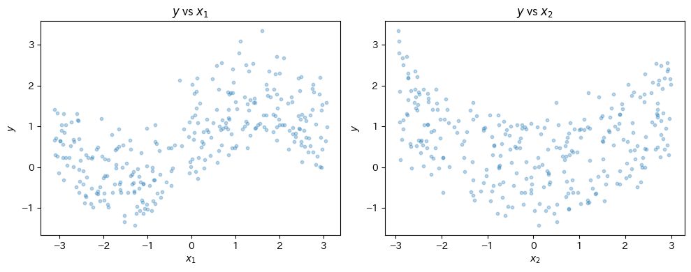
真のモデルを
として、\(n=300\) のサンプルを生成する。
n = 300
x1 = np.random.uniform(-np.pi, np.pi, n)
x2 = np.random.uniform(-3, 3, n)

f1_true = np.sin(x1)
f2_true = x2**2 / 5
y = f1_true + f2_true + np.random.normal(0, 0.3, n)

fig, axes = plt.subplots(1, 2, figsize=(10, 4))
axes[0].scatter(x1, y, alpha=0.3, s=10)
axes[0].set(xlabel="$x_1$", ylabel="$y$", title="$y$ vs $x_1$")
axes[1].scatter(x2, y, alpha=0.3, s=10)
axes[1].set(xlabel="$x_2$", ylabel="$y$", title="$y$ vs $x_2$")
plt.tight_layout()
plt.show()
スムーザーの定義#
バックフィッティングで使用するスムーザーを定義する。ここでは LOESS を用いる。frac パラメータがバンド幅に相当し、滑らかさを制御する。
def smoother(x: np.ndarray, y: np.ndarray, frac: float = 0.4) -> np.ndarray:
    """LOESS スムーザー: x の順序に沿った推定値を返す"""
    result = lowess(endog=y, exog=x, frac=frac, return_sorted=True)
    x_sorted, y_fitted = result[:, 0], result[:, 1]
    return np.interp(x, x_sorted, y_fitted)
バックフィッティングの実装#
Hastie & Tibshirani (1986) のアルゴリズムを実装する。
def backfitting(
    X: np.ndarray,
    y: np.ndarray,
    frac: float = 0.4,
    max_iter: int = 100,
    tol: float = 1e-5,
):
    """
    加法モデルのバックフィッティング推定

    Parameters
    ----------
    X : (n, p) 説明変数行列
    y : (n,) 応答変数
    frac : LOESSのバンド幅パラメータ
    max_iter : 最大イテレーション数
    tol : 収束判定閾値

    Returns
    -------
    alpha : 切片の推定値
    F : (n, p) 各 f_j の推定値
    """
    n, p = X.shape

    # 初期化
    alpha = y.mean()
    F = np.zeros((n, p))  # F[:, j] = f_j(x_{1j}), ..., f_j(x_{nj})

    for iteration in range(max_iter):
        F_old = F.copy()

        for j in range(p):
            # 部分残差: j 番目以外の関数の寄与を除く
            partial_residual = y - alpha - F.sum(axis=1) + F[:, j]

            # スムーザーを適用
            f_j_new = smoother(X[:, j], partial_residual, frac=frac)

            # 中心化(識別可能性)
            f_j_new -= f_j_new.mean()
            F[:, j] = f_j_new

        # 収束判定: 全関数の変化量の平均
        delta = np.mean((F - F_old) ** 2)
        if delta < tol:
            print(f"収束: {iteration + 1} イテレーション")
            break
    else:
        print(f"警告: {max_iter} イテレーションで収束しませんでした")

    return alpha, F
X = np.column_stack([x1, x2])
alpha_hat, F_hat = backfitting(X, y, frac=0.3)
収束: 3 イテレーション
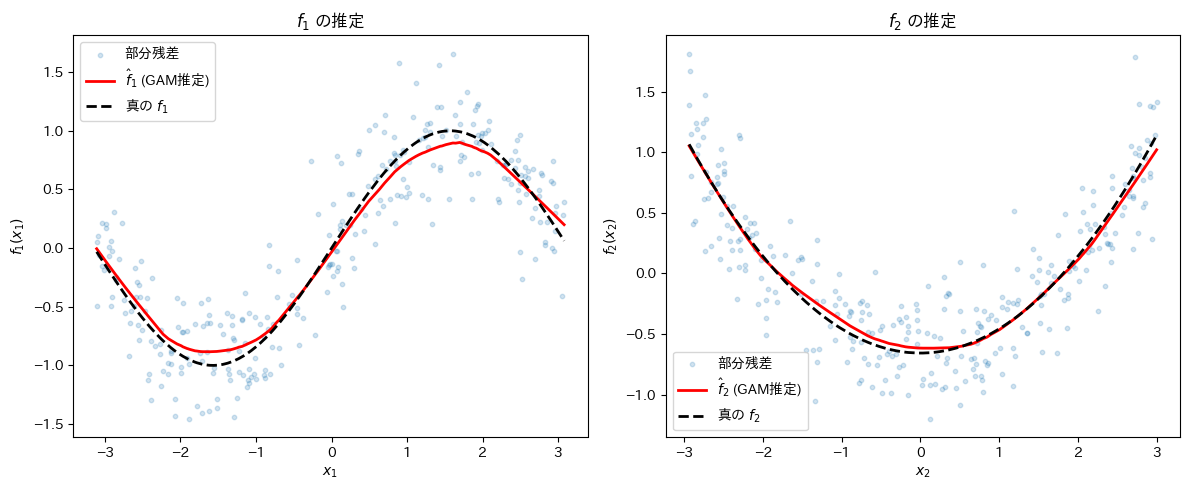
推定結果の可視化#
各 \(\hat{f}_j\) を真の関数と重ねて比較する。
fig, axes = plt.subplots(1, 2, figsize=(12, 5))

# f1 の比較
order1 = np.argsort(x1)
axes[0].scatter(x1, y - alpha_hat - F_hat[:, 1], alpha=0.2, s=10, label="部分残差")
axes[0].plot(x1[order1], F_hat[order1, 0], "r-", lw=2, label="$\\hat{f}_1$ (GAM推定)")
axes[0].plot(
    x1[order1],
    (f1_true - f1_true.mean())[order1],
    "k--",
    lw=2,
    label="真の $f_1$",
)
axes[0].set(xlabel="$x_1$", ylabel="$f_1(x_1)$", title="$f_1$ の推定")
axes[0].legend()

# f2 の比較
order2 = np.argsort(x2)
axes[1].scatter(x2, y - alpha_hat - F_hat[:, 0], alpha=0.2, s=10, label="部分残差")
axes[1].plot(x2[order2], F_hat[order2, 1], "r-", lw=2, label="$\\hat{f}_2$ (GAM推定)")
axes[1].plot(
    x2[order2],
    (f2_true - f2_true.mean())[order2],
    "k--",
    lw=2,
    label="真の $f_2$",
)
axes[1].set(xlabel="$x_2$", ylabel="$f_2(x_2)$", title="$f_2$ の推定")
axes[1].legend()

plt.tight_layout()
plt.show()
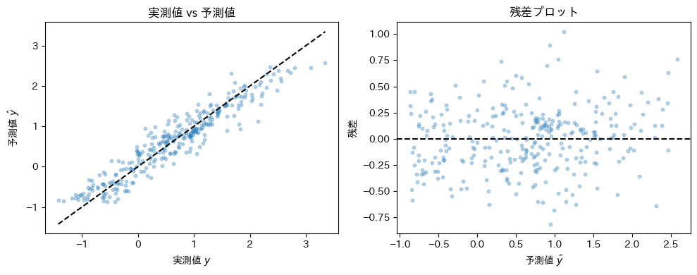
予測精度の確認#
y_pred = alpha_hat + F_hat.sum(axis=1)
residuals = y - y_pred

rmse = np.sqrt(np.mean(residuals**2))
ss_res = np.sum(residuals**2)
ss_tot = np.sum((y - y.mean())**2)
r2 = 1 - ss_res / ss_tot

print(f"RMSE : {rmse:.4f}")
print(f"R²   : {r2:.4f}")

fig, axes = plt.subplots(1, 2, figsize=(10, 4))
axes[0].scatter(y, y_pred, alpha=0.3, s=10)
lims = [min(y.min(), y_pred.min()), max(y.max(), y_pred.max())]
axes[0].plot(lims, lims, "k--")
axes[0].set(xlabel="実測値 $y$", ylabel="予測値 $\\hat{y}$", title="実測値 vs 予測値")

axes[1].scatter(y_pred, residuals, alpha=0.3, s=10)
axes[1].axhline(0, color="k", linestyle="--")
axes[1].set(xlabel="予測値 $\\hat{y}$", ylabel="残差", title="残差プロット")

plt.tight_layout()
plt.show()
RMSE : 0.3027
R²   : 0.8951
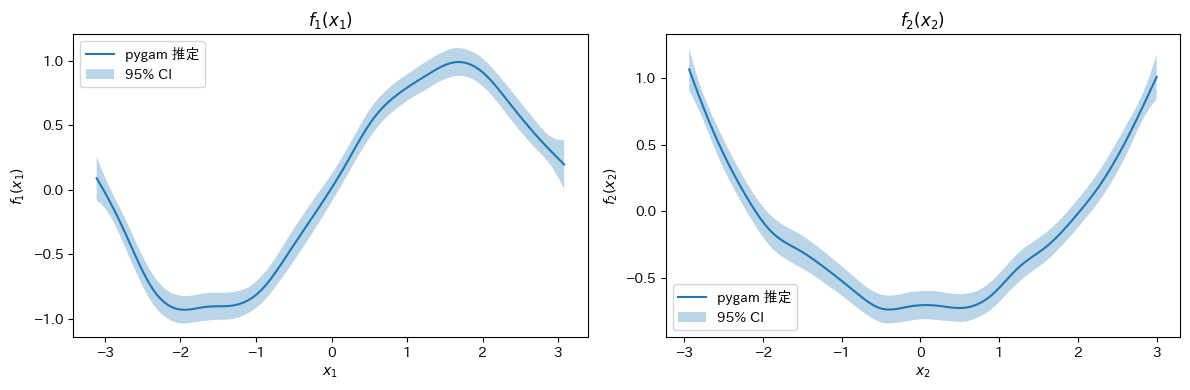
pygam を使った実装#
実用上は pygam ライブラリを使うと便利である。スプラインベースの GAM を手軽に実装できる。
try:
    from pygam import LinearGAM, s

    gam = LinearGAM(s(0) + s(1)).fit(X, y)
    print(gam.summary())

    fig, axes = plt.subplots(1, 2, figsize=(12, 4))
    titles = ["$f_1(x_1)$", "$f_2(x_2)$"]
    for i, ax in enumerate(axes):
        XX = gam.generate_X_grid(term=i)
        pdep, confi = gam.partial_dependence(term=i, X=XX, width=0.95)
        ax.plot(XX[:, i], pdep, label="pygam 推定")
        ax.fill_between(XX[:, i], confi[:, 0], confi[:, 1], alpha=0.3, label="95% CI")
        ax.set(xlabel=f"$x_{i+1}$", ylabel=titles[i], title=titles[i])
        ax.legend()
    plt.tight_layout()
    plt.show()

except ImportError:
    print("pygam がインストールされていません。`pip install pygam` でインストールできます。")
LinearGAM
=============================================== ==========================================================
Distribution:                        NormalDist Effective DoF:                                      22.834
Link Function:                     IdentityLink Log Likelihood:                                 -1079.0852
Number of Samples:                          300 AIC:                                             2205.8385
                                                AICc:                                            2210.1406
                                                GCV:                                                0.1054
                                                Scale:                                               0.091
                                                Pseudo R-Squared:                                   0.9037
==========================================================================================================
Feature Function                  Lambda               Rank         EDoF         P > x        Sig. Code
================================= ==================== ============ ============ ============ ============
s(0)                              [0.6]                20           12.3         1.11e-16     ***
s(1)                              [0.6]                20           10.6         1.11e-16     ***
intercept                                              1            0.0          1.11e-16     ***
==========================================================================================================
Significance codes:  0 '***' 0.001 '**' 0.01 '*' 0.05 '.' 0.1 ' ' 1

WARNING: Fitting splines and a linear function to a feature introduces a model identifiability problem
         which can cause p-values to appear significant when they are not.

WARNING: p-values calculated in this manner behave correctly for un-penalized models or models with
         known smoothing parameters, but when smoothing parameters have been estimated, the p-values
         are typically lower than they should be, meaning that the tests reject the null too readily.
None
/tmp/ipykernel_9829/2112680051.py:5: UserWarning: KNOWN BUG: p-values computed in this summary are likely much smaller than they should be.

Please do not make inferences based on these values!

Collaborate on a solution, and stay up to date at:
github.com/dswah/pyGAM/issues/163

  print(gam.summary())
参考文献#
Hastie, T., & Tibshirani, R. (1986). Generalized additive models. Statistical Science, 1(3), 297–310.
Buja, A., Hastie, T., & Tibshirani, R. (1989). Linear smoothers and additive models. The Annals of Statistics, 17(2), 453–510.
Hastie, T., & Tibshirani, R. (1990). Generalized Additive Models. Chapman & Hall.
Wood, S. N. (2017). Generalized Additive Models: An Introduction with R (2nd ed.). CRC Press.